ARX Time Series Model
An ARX model is a combination of an autoregressive model (AR) and an exogenous input model (X). It is used to represent the dynamics of a system and is commonly used in control engineering to model and analyze dynamic systems.
An autoregressive model is a type of statistical model that represents a time series as a linear combination of its past values and a stochastic process. It is represented by the following equation:
$$y(t) = c + a_1 y(t-1) + a_2 y(t-2) + ... + a_p y(t-p) + e(t)$$
where y(t) is the value of the time series at time t, c is a constant term, a1, a2, ..., ap are the autoregressive coefficients, y(t-1), y(t-2), ..., y(t-p) are the past values of the time series, and e(t) is a random error term.
An exogenous input model represents a time series as a linear combination of its past values and a set of exogenous (i.e., external) input variables. It is represented by the following equation:
$$y(t) = c + b_1 u_1(t) + b_2 u_2(t) + ... + b_q u_q(t) + e(t)$$
where y(t) is the value of the time series at time t, c is a constant term, u1(t), u2(t), ..., uq(t) are the exogenous input variables, and b1, b2, ..., bq are the coefficients that capture the relationship between the input variables and the output.
An ARX model is a combination of an AR model and an X model, and it is represented by the following equation:
$$y(t) = c + a_1 y(t-1) + a_2 y(t-2) +\ldots+ a_p y(t-p) \\+ b_1 u_1(t) + b_2 u_2(t) +\ldots+ b_q u_q(t) + e(t)$$
ARX time series models are a linear representation of a dynamic system in discrete time. Putting a model into ARX form is the basis for many methods in process dynamics and control analysis. Below is the time series model with a single input and single output with k as an index that refers to the time step.
$$y_{k+1} = \sum_{i=1}^{n_a} a_i y_{k-i+1} + \sum_{i=1}^{n_b} b_i u_{k-i+1}$$
With na=3, nb=2, nu=1, and ny=1 the time series model is:
$$y_{k+1} = a_1 \, y_k + a_2 \, y_{k-1} + a_3 \, y_{k-2} + b_1 \, u_k + b_2 \, u_{k-1}$$
There may also be multiple inputs and multiple outputs such as when na=1, nb=1, nu=2, and ny=2.
$$y1_{k+1} = a_{1,1} \, y1_k + b_{1,1} \, u1_k + b_{1,2} \, u2_k$$
$$y2_{k+1} = a_{1,2} \, y2_k + b_{2,1} \, u1_k + b_{2,2} \, u2_k$$
Time series models are used for identification and advanced control. It has been in use in the process industries such as chemical plants and oil refineries since the 1980s. Model predictive controllers rely on dynamic models of the process, most often linear empirical models obtained by system identification.
 Inputs: Input (u)
 Outputs: Output (y)
 Description: ARX Time Series Model
 APMonitor Usage: sys = arx
 GEKKO Usage: y,u = m.arx(p,y=[],u=[])
from gekko import GEKKO
import numpy as np
import pandas as pd
import matplotlib.pyplot as plt
# load data and parse into columns
url = 'http://apmonitor.com/do/uploads/Main/tclab_dyn_data2.txt'
data = pd.read_csv(url)
t = data['Time']
u = data['H1']
y = data['T1']
m = GEKKO()
# system identification
na = 2 # output coefficients
nb = 2 # input coefficients
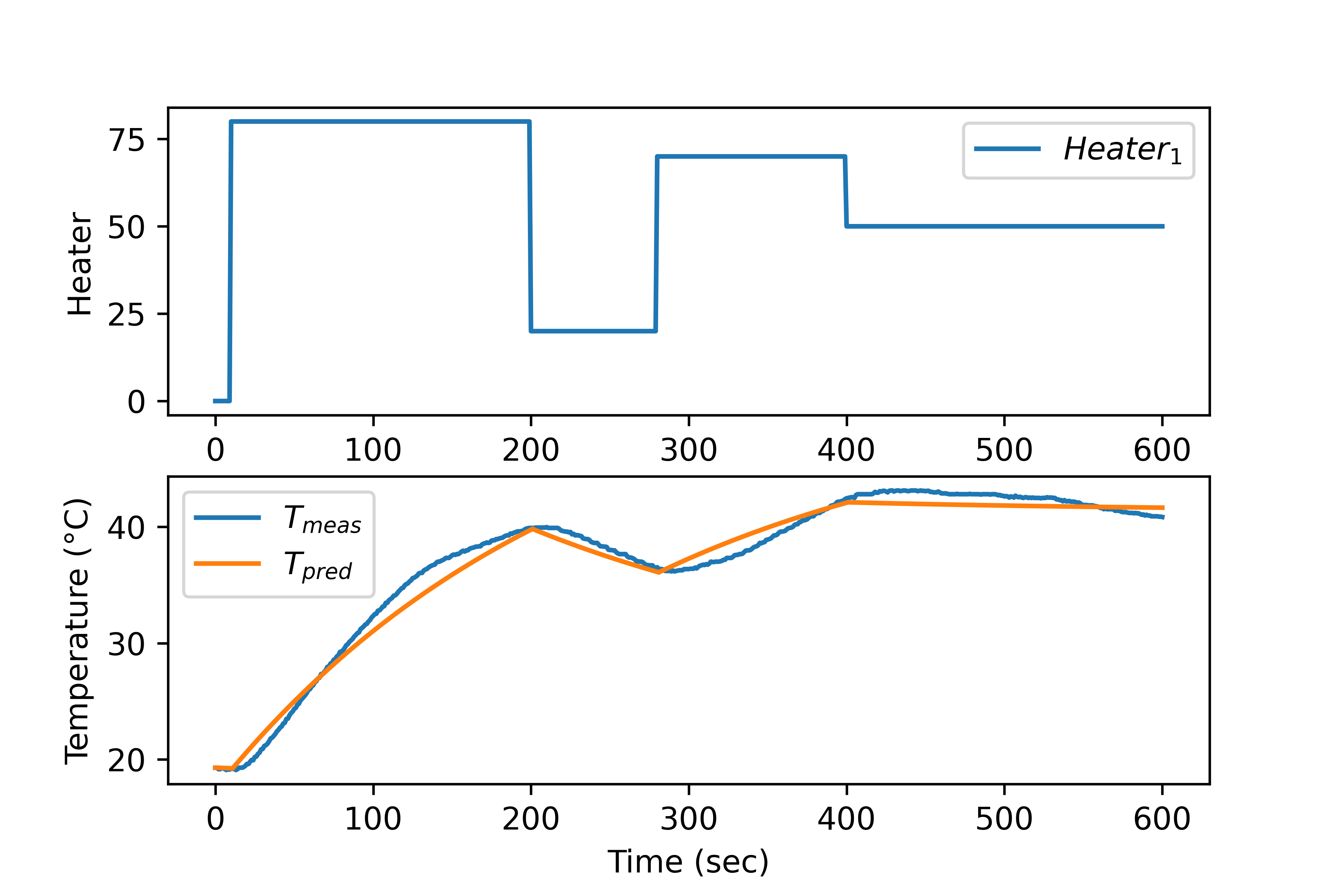
yp,p,K = m.sysid(t,u,y,na,nb,pred='meas')
plt.figure()
plt.subplot(2,1,1)
plt.plot(t,u,label=r'$Heater_1$')
plt.legend()
plt.ylabel('Heater')
plt.subplot(2,1,2)
plt.plot(t,y)
plt.plot(t,yp)
plt.legend([r'$T_{meas}$',r'$T_{pred}$'])
plt.ylabel('Temperature (°C)')
plt.xlabel('Time (sec)')
plt.show()
import numpy as np
import pandas as pd
import matplotlib.pyplot as plt
# load data and parse into columns
url = 'http://apmonitor.com/do/uploads/Main/tclab_dyn_data2.txt'
data = pd.read_csv(url)
t = data['Time']
u = data[['H1','H2']]
y = data[['T1','T2']]
m = GEKKO()
# system identification
na = 2 # output coefficients
nb = 2 # input coefficients
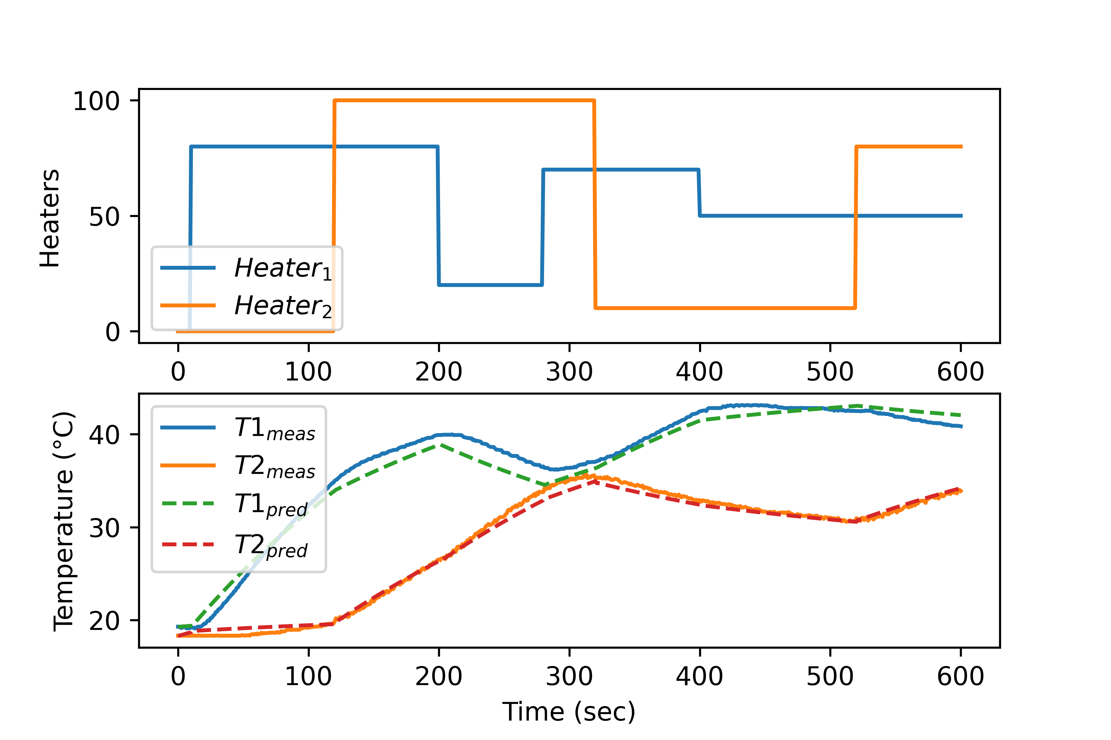
yp,p,K = m.sysid(t,u,y,na,nb,pred='meas')
plt.figure()
plt.subplot(2,1,1)
plt.plot(t,u,label=r'$Heater_1$')
plt.legend([r'$Heater_1$',r'$Heater_2$'])
plt.ylabel('Heaters')
plt.subplot(2,1,2)
plt.plot(t,y)
plt.plot(t,yp,'--')
plt.legend([r'$T1_{meas}$',r'$T2_{meas}$',\
r'$T1_{pred}$',r'$T2_{pred}$'])
plt.ylabel('Temperature (°C)')
plt.xlabel('Time (sec)')
plt.show()
These models are typically in the finite impulse response, time series, or linear state space form.

Example MPC in GEKKO with ARX Model
import time
import matplotlib.pyplot as plt
import pandas as pd
import json
# get gekko package with:
# pip install gekko
from gekko import GEKKO
# get tclab package with:
# pip install tclab
from tclab import TCLab
# Connect to Arduino
a = TCLab()
# Make an MP4 animation?
make_mp4 = False
if make_mp4:
import imageio # required to make animation
import os
try:
os.mkdir('./figures')
except:
pass
# Final time
tf = 10 # min
# number of data points (every 2 seconds)
n = tf * 30 + 1
# Percent Heater (0-100%)
Q1s = np.zeros(n)
Q2s = np.zeros(n)
# Temperatures (degC)
T1m = a.T1 * np.ones(n)
T2m = a.T2 * np.ones(n)
# Temperature setpoints
T1sp = T1m[0] * np.ones(n)
T2sp = T2m[0] * np.ones(n)
# Heater set point steps about every 150 sec
T1sp[3:] = 50.0
T2sp[40:] = 35.0
T1sp[80:] = 30.0
T2sp[120:] = 50.0
T1sp[160:] = 45.0
T2sp[200:] = 35.0
T1sp[240:] = 60.0
#########################################################
# Initialize Model
#########################################################
# load data (20 min, dt=2 sec) and parse into columns
url = 'http://apmonitor.com/do/uploads/Main/tclab_2sec.txt'
data = pd.read_csv(url)
t = data['Time']
u = data[['H1','H2']]
y = data[['T1','T2']]
# generate time-series model
m = GEKKO()
##################################################################
# system identification
na = 2 # output coefficients
nb = 2 # input coefficients
print('Identify model')
yp,p,K = m.sysid(t,u,y,na,nb,objf=10000,scale=False,diaglevel=1)
##################################################################
# plot sysid results
plt.figure()
plt.subplot(2,1,1)
plt.plot(t,u)
plt.legend([r'$H_1$',r'$H_2$'])
plt.ylabel('MVs')
plt.subplot(2,1,2)
plt.plot(t,y)
plt.plot(t,yp)
plt.legend([r'$T_{1meas}$',r'$T_{2meas}$',\
r'$T_{1pred}$',r'$T_{2pred}$'])
plt.ylabel('CVs')
plt.xlabel('Time')
plt.savefig('sysid.png')
plt.show()
##################################################################
# create control ARX model
y = m.Array(m.CV,2)
u = m.Array(m.MV,2)
m.arx(p,y,u)
# rename CVs
TC1 = y[0]
TC2 = y[1]
# rename MVs
Q1 = u[0]
Q2 = u[1]
# steady state initialization
m.options.IMODE = 1
m.solve(disp=False)
# set up MPC
m.options.IMODE = 6 # MPC
m.options.CV_TYPE = 1 # Objective type
m.options.NODES = 2 # Collocation nodes
m.options.SOLVER = 3 # IPOPT
m.time=np.linspace(0,120,61)
# Manipulated variables
Q1.STATUS = 1 # manipulated
Q1.FSTATUS = 0 # not measured
Q1.DMAX = 50.0
Q1.DCOST = 0.1
Q1.UPPER = 100.0
Q1.LOWER = 0.0
Q2.STATUS = 1 # manipulated
Q2.FSTATUS = 0 # not measured
Q2.DMAX = 50.0
Q2.DCOST = 0.1
Q2.UPPER = 100.0
Q2.LOWER = 0.0
# Controlled variables
TC1.STATUS = 1 # drive to set point
TC1.FSTATUS = 1 # receive measurement
TC1.TAU = 20 # response speed (time constant)
TC1.TR_INIT = 2 # reference trajectory
TC1.TR_OPEN = 0
TC2.STATUS = 1 # drive to set point
TC2.FSTATUS = 1 # receive measurement
TC2.TAU = 20 # response speed (time constant)
TC2.TR_INIT = 2 # dead-band
TC2.TR_OPEN = 1
##################################################################
# Create plot
plt.figure(figsize=(10,7))
plt.ion()
plt.show()
# Main Loop
start_time = time.time()
prev_time = start_time
tm = np.zeros(n)
try:
for i in range(1,n-1):
# Sleep time
sleep_max = 2.0
sleep = sleep_max - (time.time() - prev_time)
if sleep>=0.01:
time.sleep(sleep-0.01)
else:
time.sleep(0.01)
# Record time and change in time
t = time.time()
dt = t - prev_time
prev_time = t
tm[i] = t - start_time
# Read temperatures in Celsius
T1m[i] = a.T1
T2m[i] = a.T2
# Insert measurements
TC1.MEAS = T1m[i]
TC2.MEAS = T2m[i]
# Adjust setpoints
db1 = 1.0 # dead-band
TC1.SPHI = T1sp[i] + db1
TC1.SPLO = T1sp[i] - db1
db2 = 0.2
TC2.SPHI = T2sp[i] + db2
TC2.SPLO = T2sp[i] - db2
# Adjust heaters with MPC
m.solve()
if m.options.APPSTATUS == 1:
# Retrieve new values
Q1s[i+1] = Q1.NEWVAL
Q2s[i+1] = Q2.NEWVAL
# get additional solution information
with open(m.path+'//results.json') as f:
results = json.load(f)
else:
# Solution failed
Q1s[i+1] = 0.0
Q2s[i+1] = 0.0
# Write new heater values (0-100)
a.Q1(Q1s[i])
a.Q2(Q2s[i])
# Plot
plt.clf()
ax=plt.subplot(3,1,1)
ax.grid()
plt.plot(tm[0:i+1],T1sp[0:i+1]+db1,'k-',\
label=r'$T_1$ target',linewidth=3)
plt.plot(tm[0:i+1],T1sp[0:i+1]-db1,'k-',\
label=None,linewidth=3)
plt.plot(tm[0:i+1],T1m[0:i+1],'r.',label=r'$T_1$ measured')
plt.plot(tm[i]+m.time,results['v1.bcv'],'r-',\
label=r'$T_1$ predicted',linewidth=3)
plt.plot(tm[i]+m.time,results['v1.tr_hi'],'k--',\
label=r'$T_1$ trajectory')
plt.plot(tm[i]+m.time,results['v1.tr_lo'],'k--')
plt.ylabel('Temperature (degC)')
plt.legend(loc=2)
ax=plt.subplot(3,1,2)
ax.grid()
plt.plot(tm[0:i+1],T2sp[0:i+1]+db2,'k-',\
label=r'$T_2$ target',linewidth=3)
plt.plot(tm[0:i+1],T2sp[0:i+1]-db2,'k-',\
label=None,linewidth=3)
plt.plot(tm[0:i+1],T2m[0:i+1],'b.',label=r'$T_2$ measured')
plt.plot(tm[i]+m.time,results['v2.bcv'],'b-',\
label=r'$T_2$ predict',linewidth=3)
plt.plot(tm[i]+m.time,results['v2.tr_hi'],'k--',\
label=r'$T_2$ range')
plt.plot(tm[i]+m.time,results['v2.tr_lo'],'k--')
plt.ylabel('Temperature (degC)')
plt.legend(loc=2)
ax=plt.subplot(3,1,3)
ax.grid()
plt.plot([tm[i],tm[i]],[0,100],'k-',\
label='Current Time',linewidth=1)
plt.plot(tm[0:i+1],Q1s[0:i+1],'r.-',\
label=r'$Q_1$ history',linewidth=2)
plt.plot(tm[i]+m.time,Q1.value,'r-',\
label=r'$Q_1$ plan',linewidth=3)
plt.plot(tm[0:i+1],Q2s[0:i+1],'b.-',\
label=r'$Q_2$ history',linewidth=2)
plt.plot(tm[i]+m.time,Q2.value,'b-',
label=r'$Q_2$ plan',linewidth=3)
plt.plot(tm[i]+m.time[1],Q1.value[1],color='red',\
marker='.',markersize=15)
plt.plot(tm[i]+m.time[1],Q2.value[1],color='blue',\
marker='X',markersize=8)
plt.ylabel('Heaters')
plt.xlabel('Time (sec)')
plt.legend(loc=2)
plt.draw()
plt.pause(0.05)
if make_mp4:
filename='./figures/plot_'+str(i+10000)+'.png'
plt.savefig(filename)
# Turn off heaters and close connection
a.Q1(0)
a.Q2(0)
a.close()
# Save figure
plt.savefig('tclab_mpc.png')
# generate mp4 from png figures in batches of 350
if make_mp4:
images = []
iset = 0
for i in range(1,n-1):
filename='./figures/plot_'+str(i+10000)+'.png'
images.append(imageio.imread(filename))
if ((i+1)%350)==0:
imageio.mimsave('results_'+str(iset)+'.mp4', images)
iset += 1
images = []
if images!=[]:
imageio.mimsave('results_'+str(iset)+'.mp4', images)
# Allow user to end loop with Ctrl-C
except KeyboardInterrupt:
# Turn off heaters and close connection
a.Q1(0)
a.Q2(0)
a.close()
print('Shutting down')
plt.savefig('tclab_mpc.png')
# Make sure serial connection still closes when there's an error
except:
# Disconnect from Arduino
a.Q1(0)
a.Q2(0)
a.close()
print('Error: Shutting down')
plt.savefig('tclab_mpc.png')
raise
✅ Knowledge Check
1. In the ARX model equation, what role does the term e(t) play?
- Incorrect. e(t) does not represent the exogenous input variables. It is the random error term in the model.
- Incorrect. e(t) is not a coefficient. It is a term that captures the random error or noise in the model.
- Correct. e(t) is the random error term in the ARX model, capturing the unpredictable variations.
- Incorrect. e(t) is not the constant term. It is the random error term in the model.
2. What is the primary advantage of incorporating exogenous input variables in an ARX model compared to just using an AR model?
- Incorrect. Both AR and ARX models use past values, but ARX additionally incorporates exogenous input variables.
- Correct. By including exogenous inputs, the ARX model can account for external influences affecting the time series.
- Incorrect. The accuracy depends on the specific data and situation. While ARX can capture external influences, it may not always be more accurate than AR.
- Incorrect. The ARX model does use past values, similar to the AR model, but it also incorporates exogenous input variables.
Also see: