Scale Data for Machine Learning
Scaling (inputs and outputs) can improve the training process for machine learning. Certain types of classifiers do not improve with data scaling. These include Decision Trees, RandomForest, and XGBoost. Most other types of classifiers are very sensitive to scaling. The example at the end of this page shows the negative impact of unscaled data for a Neural Network Classifier. The data is scaled before training and unscaled to evaluate the performance after prediction.
A common scaling technique is to divide by the standard deviation and shift the mean to 0. Another common scaling approach is to adjust all of the data to a range of 0 to 1 or -1 to 1. Each data column is scaled individually.


There are different methods for scaling that are important based on the presence of outliers or statistical properties of the data. Two primary methods for scaling are a standard scaler (scale by the standard deviation) and a min-max (e.g. 0-1) scaler. For classifiers and regressor such as neural networks, most of the data should be between 0 and 1 or -1 and 1.
import matplotlib.pyplot as plt
# Generate a distribution
x = 0.5*np.random.randn(1000)+4
# Standard (mean=0, stdev=1) Scaler
y = (x-np.mean(x))/np.std(x)
# Min-Max (0-1) Scaler
z = (x-np.min(x))/(np.max(x)-np.min(x))
# Plot distributions
plt.figure(figsize=(8,4))
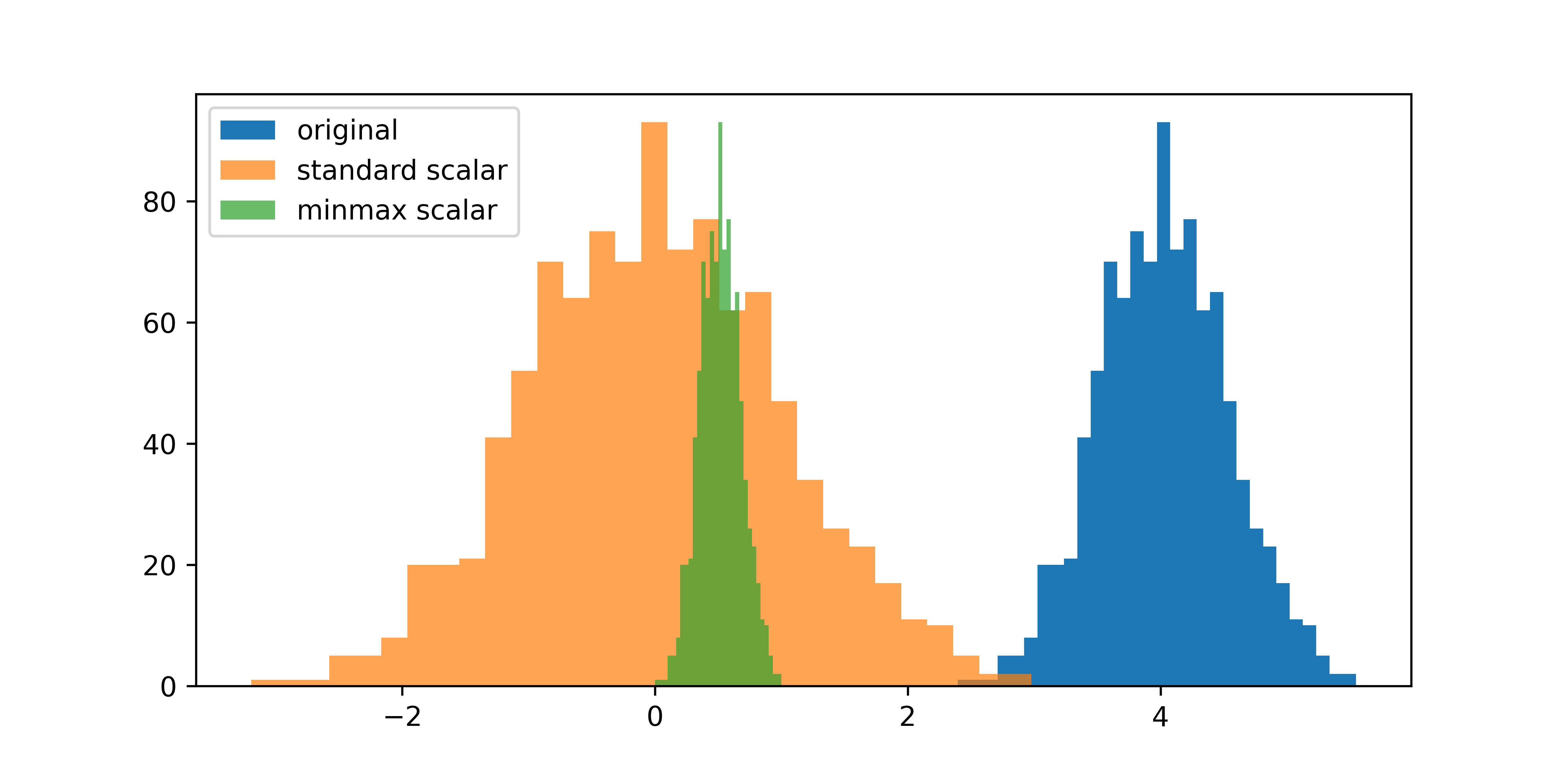
plt.hist(x, bins=30, label='original')
plt.hist(y, alpha=0.7, bins=30, label='standard scaler')
plt.hist(z, alpha=0.7, bins=30, label='minmax scaler')
plt.legend()
plt.show()
The scaled output is y and the unscaled input is x.
$$y = a \left(x-b\right)$$
The a and b adjust the original data to a transformed state.

Sample Data
Import sample data and split into training (80%) and testing (20%) sets. More information on Splitting Data is available in another module.
import pandas as pd
data = pd.read_csv('http://apmonitor.com/pds/uploads/Main/tclab_data6.txt')
data.set_index('Time',inplace=True)
# Split into train and test subsets (20% for test)
train, test = train_test_split(data, test_size=0.2, shuffle=False)
Standard Scaler
The standard scaler transforms data train into a standard normal distribution from mean=`\bar x` and standard deviation `\sigma` to a new distribution with mean=0 and unit standard deviation (`\sigma=1`).
$$y = \frac{1}{\sigma} \left(x-\bar x\right)$$
$$a=\frac{1}{\sigma},\;b=\bar x$$
The scikit-learn (sklearn) package facilitates scaling with either the fit or the fit_transform functions. The fit_transform function combined the fit and transform functions into a single operation.
s = StandardScaler()
s_train = s.fit_transform(train)
The scaling factors are available for each of the data columns.
print('Scaler mean')
print('b: ', s.mean_)
For the example problem, this produces approximately s.scale_=0.5 and s.mean_=4.0 because the original data has a standard deviation of 0.5 and a mean of 4.0. If there is another data set that needs to be transformed, the transform function uses the same scaling factors as generated from the fit_transform function.
If the original source is a Pandas dataframe, the data can be returned to a Pandas dataframe as s_train_df and s_test_df. This is needed because the fit_transform and transform functions return a Numpy array.
s_train_df = pd.DataFrame(s_train, columns=train.columns.values)
s_test_df = pd.DataFrame(s_test, columns=test.columns.values)
Min Max Scaler
An alternative to the standard scaler is the min-max scaler that adjusts all data between an upper and lower limit in the feature_range.
$$y = \frac{1}{x_{max}-x_{min}} \left(x-x_{min}\right)$$
$$a=\frac{1}{x_{max}-x_{min}},\;b=x_{min}$$
This type of scaler is useful for machine learning algorithms that require non-negative data or when the data set does not contain outliers. Outliers skew most of the data to a very narrow region within the 0-1 interval.
s = MinMaxScaler(feature_range=(0,1))
s_train = s.fit_transform(train)
s_test = s.transform(test)
The scaling factors are available for each of the data columns with scale_ and min_.
print('a: ', s.scale_)
print('Scaler minimum')
print('b: ', s.min_)
Inverse Transform
An inverse transform returns data to the original scaling. Scaled data is only for the machine learning methods that need well-conditioned data for processing. Once the training or prediction is completed, the data needs to be returned to the unscaled form for visualization or interpretation. The inverse_transform function is used to unscale the data.
$$x = \frac{y}{a}+b$$
Exercise

The Temperature Control Lab (TCLab) has two heaters (Q1 and Q2) and two temperature sensors (T1 and T2). Heater 1 (Q1) is cycled between 0% and 100% and Heater 2 Q2 is off as shown in the Equipment Monitoring exercise. A histogram plot shows the heaters and temperature distributions.
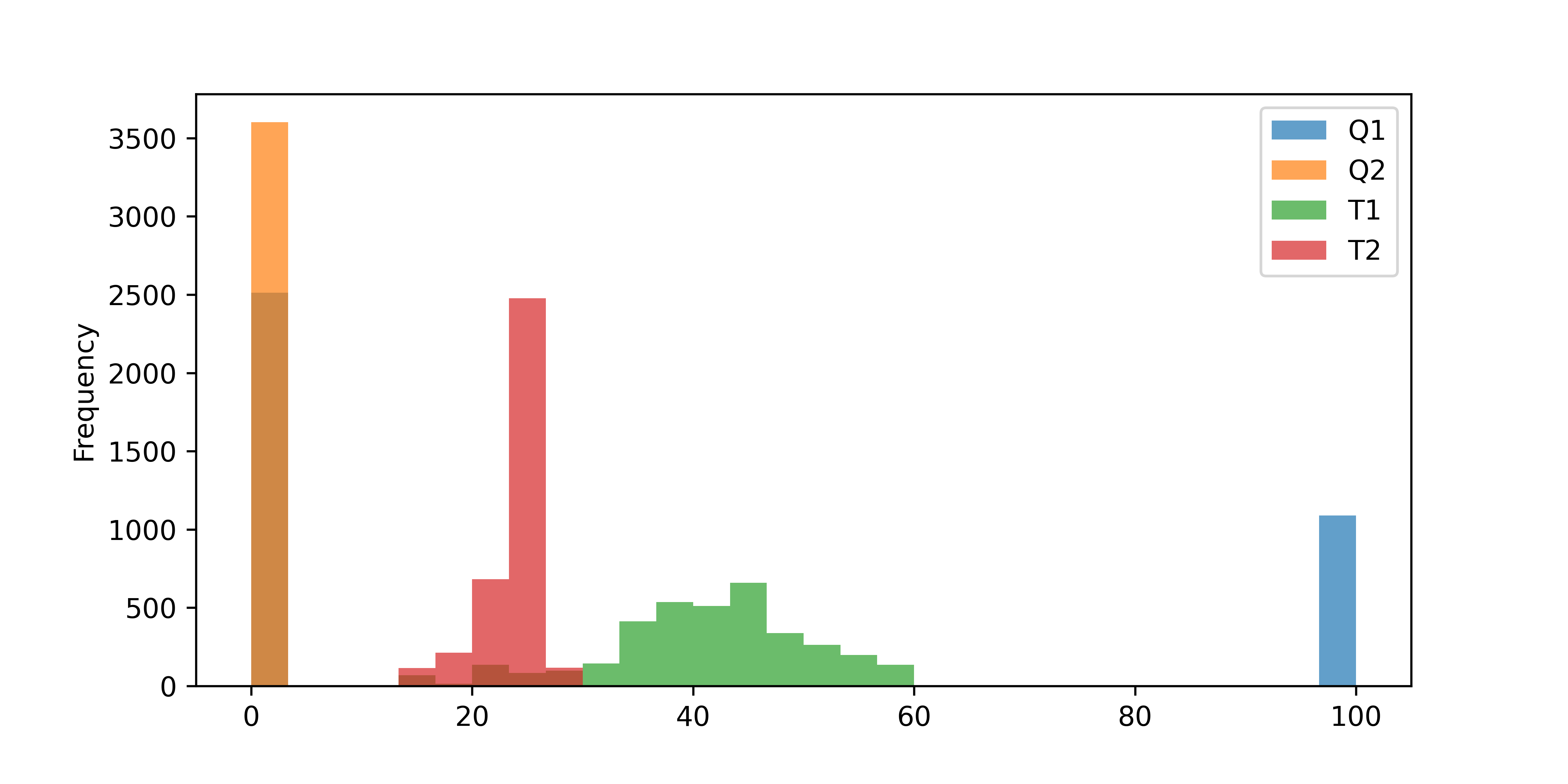
data = pd.read_csv('http://apmonitor.com/pds/uploads/Main/tclab_data6.txt')
data.set_index('Time',inplace=True)
data.plot(kind='hist',alpha=0.7,bins=30,figsize=(8,4))
Activity 1: Scale Data
Scale the TCLab data with a standard scaler and plot the distributions.
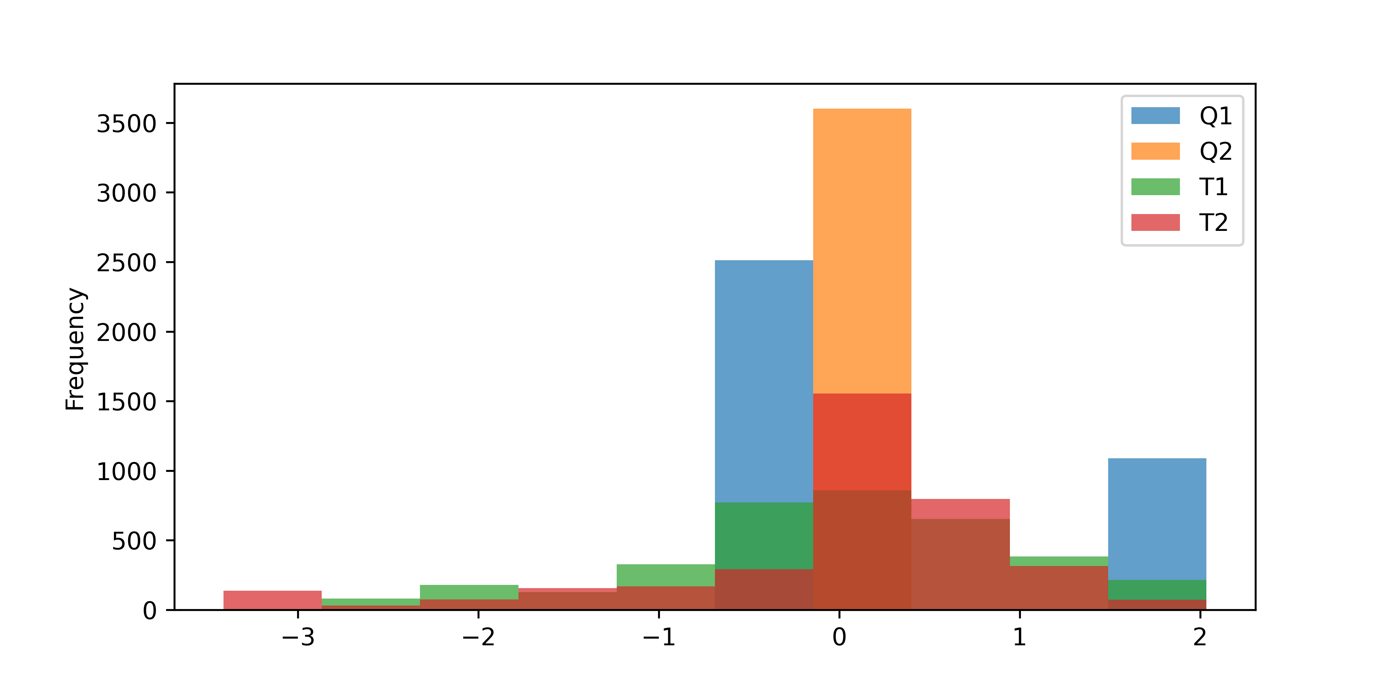
s = StandardScaler()
sdata = s.fit_transform(data)
sdata = pd.DataFrame(sdata, columns=data.columns.values, index=data.index)
sdata.plot(kind='hist',alpha=0.7,bins=10,figsize=(8,4))
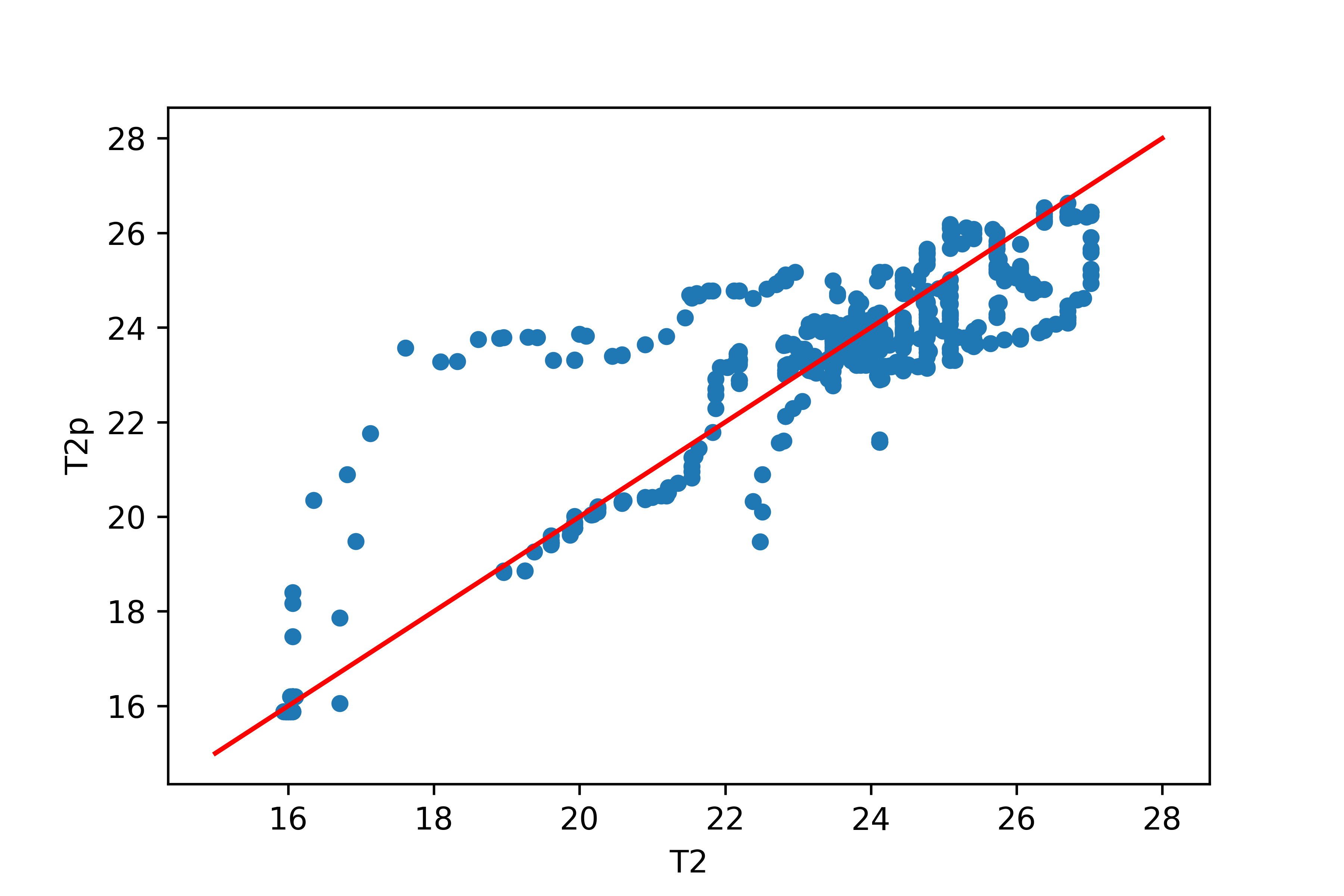
Activity 2: Neural Network with Scaled Data
Train a neural network to predict T2 (output) from Q1 and T1 (input features). Split the data into a train (80%) and test (20%) set. Create a parity plot of the predicted versus measured T2.
from sklearn.model_selection import train_test_split
import matplotlib.pyplot as plt
# split into training (80%) and testing (20%)
train, test = train_test_split(sdata, test_size=0.2, shuffle=True)
train=train.copy(); test=test.copy()
# train neural network
nn = MLPRegressor(hidden_layer_sizes=(3,3),activation='tanh',\
solver='lbfgs',max_iter=5000)
model = nn.fit(train[['Q1','T1']],train['T2'])
# test neural network
predict = test.copy()
predict['T2'] = nn.predict(test[['Q1','T1']])
# unscale data
d1 = s.inverse_transform(test)
d2 = s.inverse_transform(predict)
test_results = pd.DataFrame({'T2':d1[:,-1],'T2p':d2[:,-1]})
# plot results
test_results.plot(x='T2',y='T2p',kind='scatter')
plt.plot([15,28],[15,28],'r-')
plt.savefig('results.png',dpi=600)
plt.show()
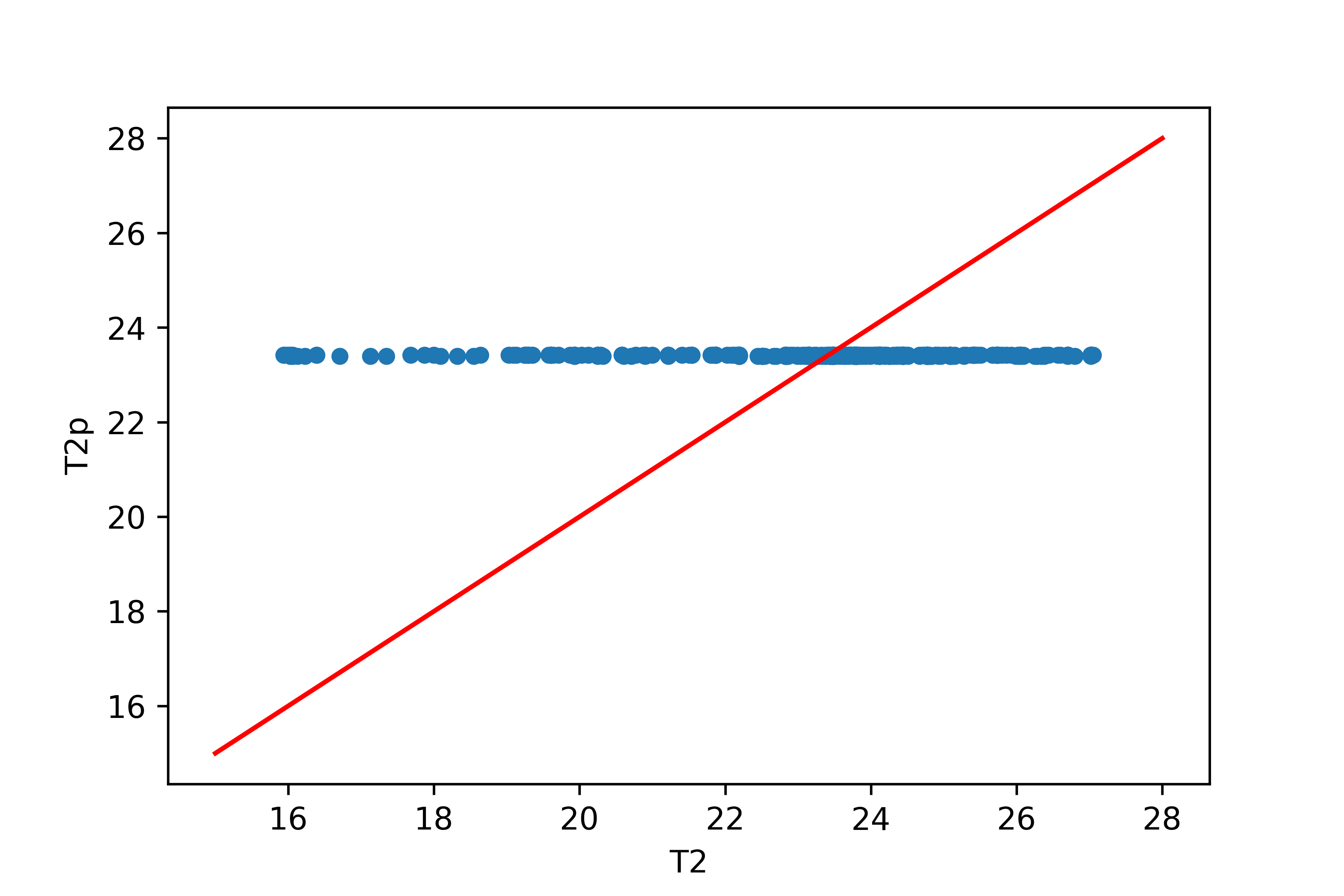
Activity 3: Neural Network with Unscaled Data
Repeat Activity 2 but use unscaled data instead of scaled data to perform the regression. Evaluate the neural network performance with a parity plot of the predicted and measured T2 on the test set.
from sklearn.model_selection import train_test_split
import matplotlib.pyplot as plt
import pandas as pd
data = pd.read_csv('http://apmonitor.com/pds/uploads/Main/tclab_data6.txt')
data.set_index('Time',inplace=True)
# split into training (80%) and testing (20%)
train, test = train_test_split(data, test_size=0.2, shuffle=True)
train=train.copy(); test=test.copy()
# train neural network
nn = MLPRegressor(hidden_layer_sizes=(3,3),activation='tanh',\
solver='lbfgs',max_iter=5000)
model = nn.fit(train[['Q1','T1']],train['T2'])
# test neural network
test['T2p'] = nn.predict(test[['Q1','T1']])
# plot results
test.plot(x='T2',y='T2p',kind='scatter')
plt.plot([15,28],[15,28],'r-')
plt.show()
✅ Knowledge Check
1. Which of the following classifiers is sensitive to data scaling?
- Correct. Neural Network Classifier is very sensitive to scaling. As mentioned in the example, the negative impact of unscaled data on a Neural Network Classifier is evident.
- Incorrect. Decision Trees do not improve with data scaling and aren't sensitive to it.
- Incorrect. RandomForest, like Decision Trees, do not improve with data scaling.
2. What is a common technique for data scaling?
- Incorrect. Multiplying every value by 2 is not a standard technique for data scaling.
- Incorrect. The common technique mentioned is shifting the mean to 0, not 3.
- Correct. One of the common techniques mentioned is adjusting all of the data to a range of 0 to 1 or -1 to 1 (Min/Max Scalar) or shifting to mean of 0 and standard deviation of 1 (Standard Scalar).
- Incorrect. Taking the absolute value is not a common technique for data scaling.