LSTM Networks
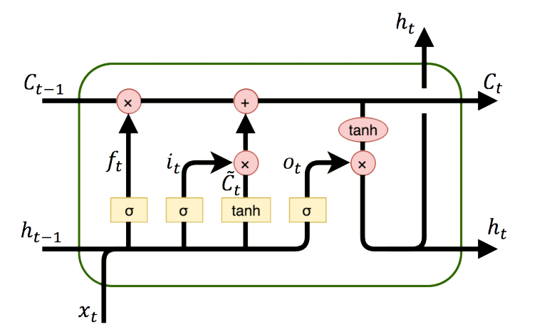
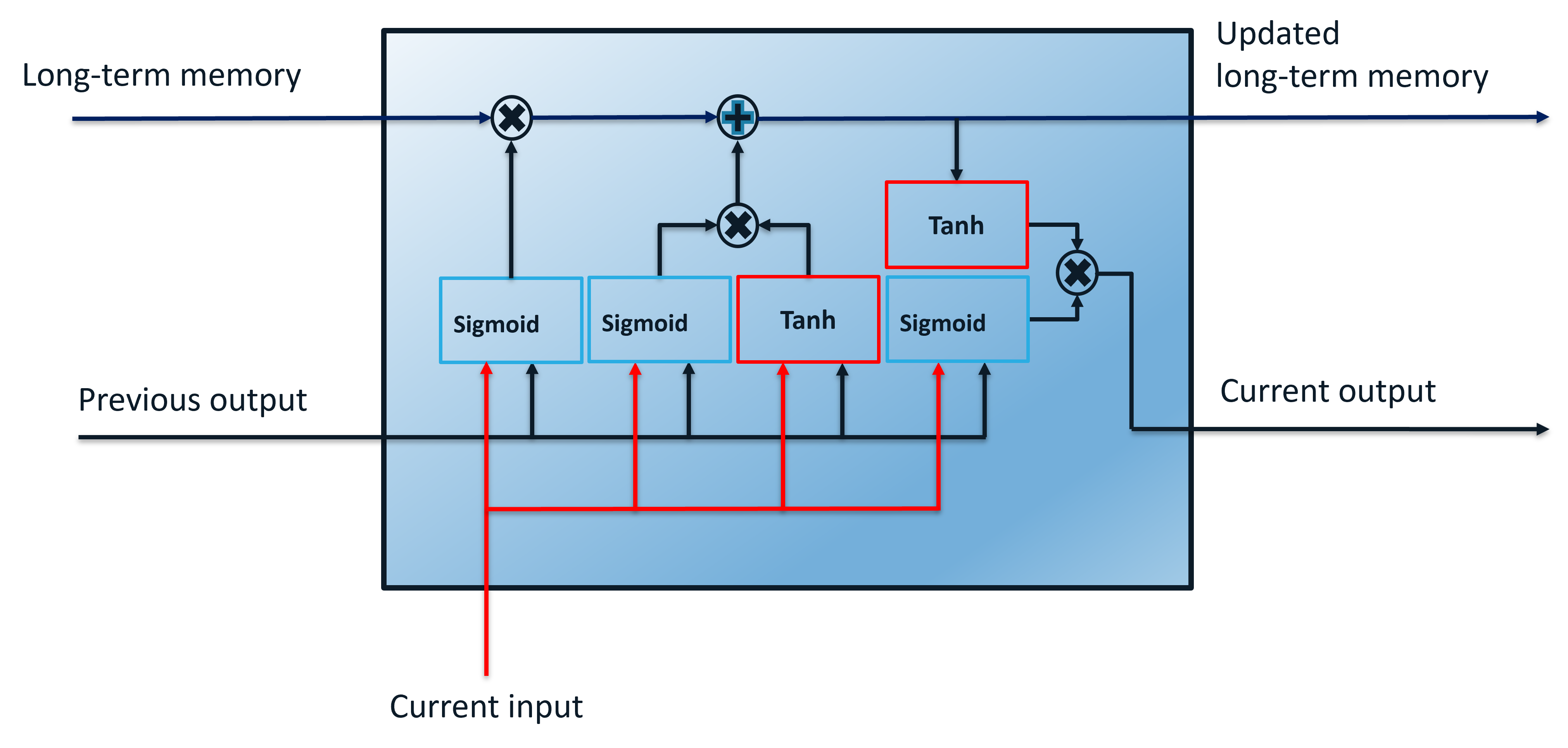
LSTM (Long Short Term Memory) networks are a special type of RNN (Recurrent Neural Network) that is structured to remember and predict based on long-term dependencies that are trained with time-series data. An LSTM repeating module has four interacting components.
The LSTM is trained (parameters adjusted) with an input window of prior data and minimized difference between the predicted and next measured value. Sequential methods predict just one next value based on the window of prior data. When there is contextual data (before and after) the desired prediction point, a Convolutional Neural Network (CNN) may improve performance with fewer resources to train and deploy the network.
Data Preparation
Data preparation for LSTM networks involves consolidation, cleansing, separating the input window and output, scaling, and data division for training and validation.
- Consolidation - consolidation is the process of combining disparate data (Excel spreadsheet, PDF report, database, cloud storage) into a single repository.
- Data Cleansing - bad data should be removed and may include outliers, missing entries, failed sensors, or other types of missing or corrupted information.
- Inputs and Outputs - data is separated into inputs (prior time-series window) and outputs (predicted next value). The inputs are fed into a series of functions to produce the output prediction. The squared difference between the predicted output and the measured output is a typical loss (objective) function for fitting.
- Scaling - scaling all data (inputs and outputs) to a range of 0-1 can improve the training process.
- Training and Validation - data is divided into training (e.g. 80%) and validation (e.g. 20%) sets so that the model fit can be evaluated independently of the training. Cross-validation is an approach to divide the training data into multiple sets that are fit separately. The parameter consistency is compared between the multiple models.
Data Generation and Preparation
import matplotlib.pyplot as plt
# Generate data
n = 500
t = np.linspace(0,20.0*np.pi,n)
X = np.sin(t) # X is already between -1 and 1, scaling normally needed
Once the data is created, it is converted to a form that can be used by Keras and Tensorflow for training and prediction.
window = 10
# Split 80/20 into train/test data
last = int(n/5.0)
Xtrain = X[:-last]
Xtest = X[-last-window:]
# Store window number of points as a sequence
xin = []
next_X = []
for i in range(window,len(Xtrain)):
xin.append(Xtrain[i-window:i])
next_X.append(Xtrain[i])
# Reshape data to format for LSTM
xin, next_X = np.array(xin), np.array(next_X)
xin = xin.reshape(xin.shape[0], xin.shape[1], 1)
LSTM Model Build
An LSTM network relates the input data window to outputs with layers. Instead of just one layer, LSTMs often have multiple layers.
from keras.layers import Dense
from keras.layers import LSTM
from keras.layers import Dropout
# Initialize LSTM model
m = Sequential()
m.add(LSTM(units=50, return_sequences=True, input_shape=(xin.shape[1],1)))
m.add(Dropout(0.2))
m.add(LSTM(units=50))
m.add(Dropout(0.2))
m.add(Dense(units=1))
m.compile(optimizer = 'adam', loss = 'mean_squared_error')
LSTM Model Training
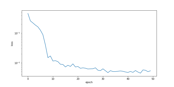
history = m.fit(xin, next_X, epochs = 50, batch_size = 50,verbose=0)
plt.figure()
plt.ylabel('loss'); plt.xlabel('epoch')
plt.semilogy(history.history['loss'])
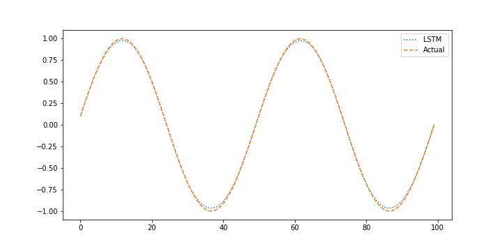
LSTM Prediction Validation
The validation test set assesses the ability of the neural network to predict based on new conditions that were not part of the training set. The validation is performed with the last 20% of the data that was separated from the beginning 80% of data.
xin = []
next_X1 = []
for i in range(window,len(Xtest)):
xin.append(Xtest[i-window:i])
next_X1.append(Xtest[i])
# Reshape data to format for LSTM
xin, next_X1 = np.array(xin), np.array(next_X1)
xin = xin.reshape((xin.shape[0], xin.shape[1], 1))
# Predict the next value (1 step ahead)
X_pred = m.predict(xin)
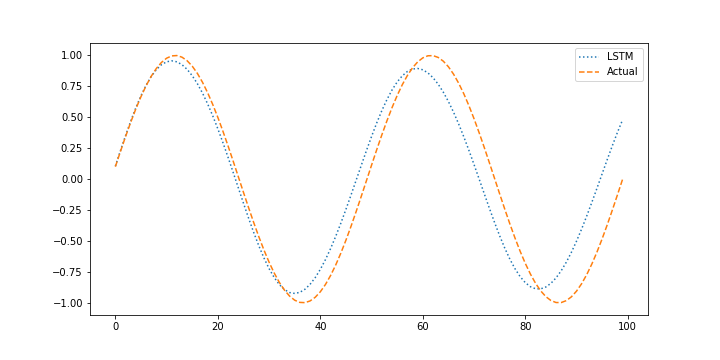
# Plot prediction vs actual for test data
plt.figure()
plt.plot(X_pred,':',label='LSTM')
plt.plot(next_X1,'--',label='Actual')
plt.legend()
LSTM Forecast Validation
When performing the validation it is also important to determine how the model performs with without measurements when it uses prior predictions to predict the next outcome. This is important to determine how well the model performs in a predictive application such as model predictive control where the model is projected forward over the control horizon to determine the sequence of optimal manipulated variable moves and possible future constraint violation. Generating predictions without measurement feedback is a forecast.
X_pred = Xtest.copy()
for i in range(window,len(X_pred)):
xin = X_pred[i-window:i].reshape((1, window, 1))
X_pred[i] = m.predict(xin)
# Plot prediction vs actual for test data
plt.figure()
plt.plot(X_pred[window:],':',label='LSTM')
plt.plot(next_X1,'--',label='Actual')
plt.legend()
import matplotlib.pyplot as plt
from keras.models import Sequential
from keras.layers import Dense
from keras.layers import LSTM
from keras.layers import Dropout
# Generate data
n = 500
t = np.linspace(0,20.0*np.pi,n)
X = np.sin(t) # X is already between -1 and 1, scaling normally needed
# Set window of past points for LSTM model
window = 10
# Split 80/20 into train/test data
last = int(n/5.0)
Xtrain = X[:-last]
Xtest = X[-last-window:]
# Store window number of points as a sequence
xin = []
next_X = []
for i in range(window,len(Xtrain)):
xin.append(Xtrain[i-window:i])
next_X.append(Xtrain[i])
# Reshape data to format for LSTM
xin, next_X = np.array(xin), np.array(next_X)
xin = xin.reshape(xin.shape[0], xin.shape[1], 1)
# Initialize LSTM model
m = Sequential()
m.add(LSTM(units=50, return_sequences=True, input_shape=(xin.shape[1],1)))
m.add(Dropout(0.2))
m.add(LSTM(units=50))
m.add(Dropout(0.2))
m.add(Dense(units=1))
m.compile(optimizer = 'adam', loss = 'mean_squared_error')
# Fit LSTM model
history = m.fit(xin, next_X, epochs = 50, batch_size = 50,verbose=0)
plt.figure()
plt.ylabel('loss'); plt.xlabel('epoch')
plt.semilogy(history.history['loss'])
# Store "window" points as a sequence
xin = []
next_X1 = []
for i in range(window,len(Xtest)):
xin.append(Xtest[i-window:i])
next_X1.append(Xtest[i])
# Reshape data to format for LSTM
xin, next_X1 = np.array(xin), np.array(next_X1)
xin = xin.reshape((xin.shape[0], xin.shape[1], 1))
# Predict the next value (1 step ahead)
X_pred = m.predict(xin)
# Plot prediction vs actual for test data
plt.figure()
plt.plot(X_pred,':',label='LSTM')
plt.plot(next_X1,'--',label='Actual')
plt.legend()
# Using predicted values to predict next step
X_pred = Xtest.copy()
for i in range(window,len(X_pred)):
xin = X_pred[i-window:i].reshape((1, window, 1))
X_pred[i] = m.predict(xin)
# Plot prediction vs actual for test data
plt.figure()
plt.plot(X_pred[window:],':',label='LSTM')
plt.plot(next_X1,'--',label='Actual')
plt.legend()
plt.show()
MATLAB Live Script

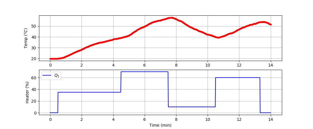
Exercise 1: LSTM Digital Twin
Develop a model of the dynamic temperature response of the TCLab and compare the LSTM model prediction to a second-order linear differential equation solution. Use the 4 hours of dynamic data from a TCLab (14400 data points = 1 second sample rate for 4 hours) for training and generate new data (840 data points = 1 second sample rate for 14 min) for validation (see sample validation data).
import numpy as np
import matplotlib.pyplot as plt
import pandas as pd
import tclab
import time
n = 840 # Number of second time points (14 min)
tm = np.linspace(0,n,n+1) # Time values
lab = tclab.TCLab()
T1 = [lab.T1]
T2 = [lab.T2]
Q1 = np.zeros(n+1)
Q2 = np.zeros(n+1)
Q1[30:] = 35.0
Q1[270:] = 70.0
Q1[450:] = 10.0
Q1[630:] = 60.0
Q1[800:] = 0.0
for i in range(n):
lab.Q1(Q1[i])
lab.Q2(Q2[i])
time.sleep(1)
print(Q1[i],lab.T1)
T1.append(lab.T1)
T2.append(lab.T2)
lab.close()
# Save data file
data = np.vstack((tm,Q1,Q2,T1,T2)).T
np.savetxt('tclab_data.csv',data,delimiter=',',\
header='Time,Q1,Q2,T1,T2',comments='')
# Create Figure
plt.figure(figsize=(10,7))
ax = plt.subplot(2,1,1)
ax.grid()
plt.plot(tm/60.0,T1,'r.',label=r'$T_1$')
plt.ylabel(r'Temp ($^oC$)')
ax = plt.subplot(2,1,2)
ax.grid()
plt.plot(tm/60.0,Q1,'b-',label=r'$Q_1$')
plt.ylabel(r'Heater (%)')
plt.xlabel('Time (min)')
plt.legend()
plt.savefig('tclab_data.png')
plt.show()
Use the measured temperature and heater values to predict the next temperature value with an LSTM model. Validate the model with a new data set in a predictive and forecast mode. The predictive mode predicts one step ahead while the forecast does not use temperature measurements to generate the predictions.
Solution with LSTM Model
The LSTM model is trained with the TCLab 4 hours data set for 10 epochs. The loss function decreases for the first few epochs and then does not significantly change after that.
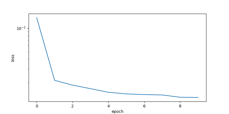
The model predictions have good agreement with the measurements. The next steps are to perform validation to determine the predictive capability of the model on a different data set.
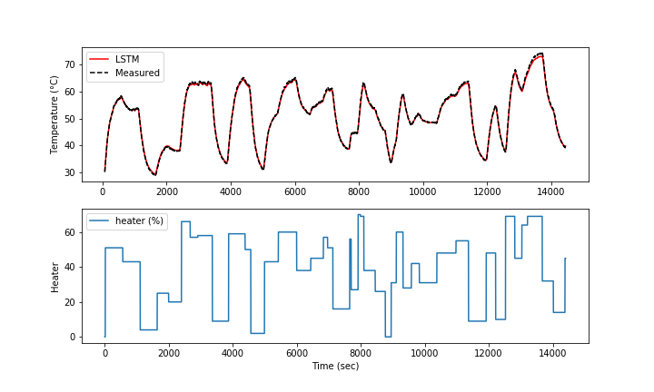
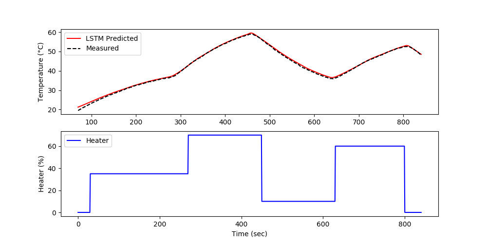
The validation shows the performance on data that was not used in the training. In this case, a separate data file is generated versus splitting the training and test data.
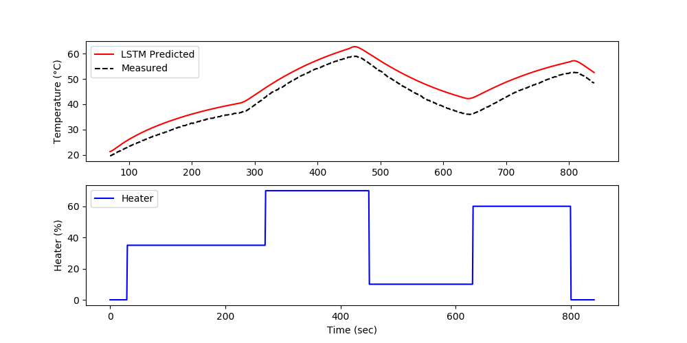
The forecast is generated by using the prior LSTM predictions to predict future temperatures. The measurements are only used for initializing the predictions and then predictions are used to predict following values.
import numpy as np
import matplotlib.pyplot as plt
from sklearn.preprocessing import MinMaxScaler
import time
# For LSTM model
from keras.models import Sequential
from keras.layers import Dense
from keras.layers import LSTM
from keras.layers import Dropout
from keras.callbacks import EarlyStopping
from keras.models import load_model
# Load training data
file = 'http://apmonitor.com/do/uploads/Main/tclab_dyn_data3.txt'
train = pd.read_csv(file)
# Scale features
s1 = MinMaxScaler(feature_range=(-1,1))
Xs = s1.fit_transform(train[['T1','Q1']])
# Scale predicted value
s2 = MinMaxScaler(feature_range=(-1,1))
Ys = s2.fit_transform(train[['T1']])
# Each time step uses last 'window' to predict the next change
window = 70
X = []
Y = []
for i in range(window,len(Xs)):
X.append(Xs[i-window:i,:])
Y.append(Ys[i])
# Reshape data to format accepted by LSTM
X, Y = np.array(X), np.array(Y)
# create and train LSTM model
# Initialize LSTM model
model = Sequential()
model.add(LSTM(units=50, return_sequences=True, \
input_shape=(X.shape[1],X.shape[2])))
model.add(Dropout(0.2))
model.add(LSTM(units=50, return_sequences=True))
model.add(Dropout(0.2))
model.add(LSTM(units=50))
model.add(Dropout(0.2))
model.add(Dense(units=1))
model.compile(optimizer = 'adam', loss = 'mean_squared_error',\
metrics = ['accuracy'])
# Allow for early exit
es = EarlyStopping(monitor='loss',mode='min',verbose=1,patience=10)
# Fit (and time) LSTM model
t0 = time.time()
history = model.fit(X, Y, epochs = 10, batch_size = 250, callbacks=[es], verbose=1)
t1 = time.time()
print('Runtime: %.2f s' %(t1-t0))
# Plot loss
plt.figure(figsize=(8,4))
plt.semilogy(history.history['loss'])
plt.xlabel('epoch'); plt.ylabel('loss')
plt.savefig('tclab_loss.png')
model.save('model.h5')
# Verify the fit of the model
Yp = model.predict(X)
# un-scale outputs
Yu = s2.inverse_transform(Yp)
Ym = s2.inverse_transform(Y)
plt.figure(figsize=(10,6))
plt.subplot(2,1,1)
plt.plot(train['Time'][window:],Yu,'r-',label='LSTM')
plt.plot(train['Time'][window:],Ym,'k--',label='Measured')
plt.ylabel('Temperature (°C)')
plt.legend()
plt.subplot(2,1,2)
plt.plot(train['Q1'],label='heater (%)')
plt.legend()
plt.xlabel('Time (sec)'); plt.ylabel('Heater')
plt.savefig('tclab_fit.png')
# Load model
v = load_model('model.h5')
# Load training data
test = pd.read_csv('http://apmonitor.com/pdc/uploads/Main/tclab_data4.txt')
Xt = test[['T1','Q1']].values
Yt = test[['T1']].values
Xts = s1.transform(Xt)
Yts = s2.transform(Yt)
Xti = []
Yti = []
for i in range(window,len(Xts)):
Xti.append(Xts[i-window:i,:])
Yti.append(Yts[i])
# Reshape data to format accepted by LSTM
Xti, Yti = np.array(Xti), np.array(Yti)
# Verify the fit of the model
Ytp = model.predict(Xti)
# un-scale outputs
Ytu = s2.inverse_transform(Ytp)
Ytm = s2.inverse_transform(Yti)
plt.figure(figsize=(10,6))
plt.subplot(2,1,1)
plt.plot(test['Time'][window:],Ytu,'r-',label='LSTM Predicted')
plt.plot(test['Time'][window:],Ytm,'k--',label='Measured')
plt.legend()
plt.ylabel('Temperature (°C)')
plt.subplot(2,1,2)
plt.plot(test['Time'],test['Q1'],'b-',label='Heater')
plt.xlabel('Time (sec)'); plt.ylabel('Heater (%)')
plt.legend()
plt.savefig('tclab_validate.png')
# Using predicted values to predict next step
Xtsq = Xts.copy()
for i in range(window,len(Xtsq)):
Xin = Xtsq[i-window:i].reshape((1, window, 2))
Xtsq[i][0] = v.predict(Xin)
Yti[i-window] = Xtsq[i][0]
#Ytu = (Yti - s2.min_[0])/s2.scale_[0]
Ytu = s2.inverse_transform(Yti)
plt.figure(figsize=(10,6))
plt.subplot(2,1,1)
plt.plot(test['Time'][window:],Ytu,'r-',label='LSTM Predicted')
plt.plot(test['Time'][window:],Ytm,'k--',label='Measured')
plt.legend()
plt.ylabel('Temperature (°C)')
plt.subplot(2,1,2)
plt.plot(test['Time'],test['Q1'],'b-',label='Heater')
plt.xlabel('Time (sec)'); plt.ylabel('Heater (%)')
plt.legend()
plt.savefig('tclab_forecast.png')
plt.show()
Solution with 2nd-Order Model
A second order model is aligned with data by adjusting unknown parameters to minimize the sum of squared errors. The adjusted parameters are `K_1`, `\tau_1`, and `\tau_2`.
$$\min \sum_{i=1}^{n} \left(T_{C1,meas,i}-T_{C1,pred,i}\right)^2$$
$$\tau_1 \frac{dT_{H1}}{dt} + \left(T_{H1}-T_a\right) = K_1 \, Q_1$$
$$\tau_2 \frac{dT_{C1}}{dt} + T_{C1} = T_{H1}$$
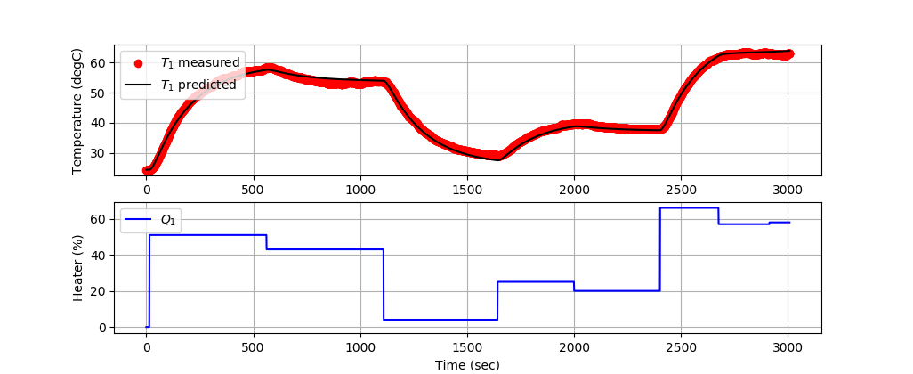
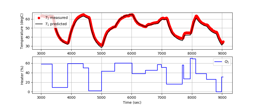
The first 3000 data points train the model and the next 6000 data points validate the model predictions on data that has not been used for training.
Training 2nd-Order Model
Validating 2nd-Order Model
import matplotlib.pyplot as plt
from gekko import GEKKO
import pandas as pd
file = 'http://apmonitor.com/do/uploads/Main/tclab_dyn_data3.txt'
data = pd.read_csv(file)
# subset for training
n = 3000
tm = data['Time'][0:n].values
Q1s = data['Q1'][0:n].values
T1s = data['T1'][0:n].values
m = GEKKO()
m.time = tm
# Parameters to Estimate
K1 = m.FV(value=0.5,lb=0.1,ub=1.0)
tau1 = m.FV(value=150,lb=50,ub=250)
tau2 = m.FV(value=15,lb=10,ub=20)
K1.STATUS = 1
tau1.STATUS = 1
tau2.STATUS = 1
# Model Inputs
Q1 = m.Param(value=Q1s)
Ta = m.Param(value=23.0) # degC
T1m = m.Param(T1s)
# Model Variables
TH1 = m.Var(value=T1s[0])
TC1 = m.Var(value=T1s)
# Objective Function
m.Minimize((T1m-TC1)**2)
# Equations
m.Equation(tau1 * TH1.dt() + (TH1-Ta) == K1*Q1)
m.Equation(tau2 * TC1.dt() + TC1 == TH1)
# Global Options
m.options.IMODE = 5 # MHE
m.options.EV_TYPE = 2 # Objective type
m.options.NODES = 2 # Collocation nodes
m.options.SOLVER = 3 # IPOPT
# Predict Parameters and Temperatures
m.solve()
# Create plot
plt.figure(figsize=(10,7))
ax=plt.subplot(2,1,1)
ax.grid()
plt.plot(tm,T1s,'ro',label=r'$T_1$ measured')
plt.plot(tm,TC1.value,'k-',label=r'$T_1$ predicted')
plt.ylabel('Temperature (degC)')
plt.legend(loc=2)
ax=plt.subplot(2,1,2)
ax.grid()
plt.plot(tm,Q1s,'b-',label=r'$Q_1$')
plt.ylabel('Heater (%)')
plt.xlabel('Time (sec)')
plt.legend(loc='best')
# Print optimal values
print('K1: ' + str(K1.newval))
print('tau1: ' + str(tau1.newval))
print('tau2: ' + str(tau2.newval))
# Save and show figure
plt.savefig('tclab_2nd_order_fit.png')
# Validation
tm = data['Time'][n:3*n].values
Q1s = data['Q1'][n:3*n].values
T1s = data['T1'][n:3*n].values
v = GEKKO()
v.time = tm
# Parameters to Estimate
K1 = K1.newval
tau1 = tau1.newval
tau2 = tau2.newval
Q1 = v.Param(value=Q1s)
Ta = v.Param(value=23.0) # degC
TH1 = v.Var(value=T1s[0])
TC1 = v.Var(value=T1s[0])
v.Equation(tau1 * TH1.dt() + (TH1-Ta) == K1*Q1)
v.Equation(tau2 * TC1.dt() + TC1 == TH1)
v.options.IMODE = 4 # Simulate
v.options.NODES = 2 # Collocation nodes
v.options.SOLVER = 1
# Predict Parameters and Temperatures
v.solve(disp=True)
# Create plot
plt.figure(figsize=(10,7))
ax=plt.subplot(2,1,1)
ax.grid()
plt.plot(tm,T1s,'ro',label=r'$T_1$ measured')
plt.plot(tm,TC1.value,'k-',label=r'$T_1$ predicted')
plt.ylabel('Temperature (degC)')
plt.legend(loc=2)
ax=plt.subplot(2,1,2)
ax.grid()
plt.plot(tm,Q1s,'b-',label=r'$Q_1$')
plt.ylabel('Heater (%)')
plt.xlabel('Time (sec)')
plt.legend(loc='best')
# Save and show figure
plt.savefig('tclab_2nd_order_validate.png')
plt.show()
Exercise 2: LSTM Replaces PID and MPC
See Automation with LSTM for a case study on replacing PID control or Model Predictive Control (MPC) with an LSTM network.

✅ Knowledge Check
1. Which of the following is NOT a step in data preparation for LSTM networks?
- Incorrect. Consolidation is the process of combining disparate data into a single repository.
- Incorrect. Scaling all data to a range of 0-1 can improve the training process.
- Correct. Data Duplication is not mentioned as a step in data preparation for LSTM networks.
- Incorrect. Data Cleansing involves removing bad data, including outliers and missing entries.
2. What is the purpose of using Dropout layers in the LSTM model?
- Incorrect. The purpose of consolidation is not related to Dropout layers but to combining disparate data sources.
- Incorrect. The memory capacity of LSTM is not directly enhanced by Dropout layers.
- Incorrect. Dropout layers do not inherently speed up the training process.
- Correct. Dropout layers are used to prevent overfitting by randomly setting a fraction of input units to 0 at each update during training time.
Further Reading
- Phi, M. Illustrated Guide to LSTM’s and GRU’s: A step by step explanation, Towards Data Science, Sept 2018.
- Brownlee, J. Multi-Step LSTM Time Series Forecasting Models for Power Usage, Machine Learning Mastery, Oct 2018.
- Olah, C., Understanding LSTM Networks, Colah's blog, Aug 2015.