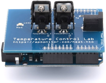
TCLab Second Order Regression
 |  |  |  |  |
|---|
Objective: Develop an adaptive regression that recalculates parameters of a second order model as new data is measured. Discuss how adaptive parameter regression could be used to adapt a PID controller with gain scheduling.
Gain scheduling is practice of changing the PID control gain based on many factors including time, distance from setpoint, operating regime such as startup or shutdown, based on a process variable zone. Gain scheduling is may be used for nonlinear processes where the process gain or time constant is different at high or low values. Gain scheduling is one example of adaptive control that includes other strategies that sense and modify control behavior based on observed system response. The purpose of this exercise is to adaptively estimate a second-order model as new data arrives, not as a batch regression when all of the data is collected.
To solve the adaptive parameter regression with either Scipy.opitimize.minimize or Python Gekko, modify the function to include the analytic solution for an overdamped 2nd order response to a step input of 80%.
def model(T0,t,M,Kp,taus,zeta):
# T0 = initial T
# t = time
# M = magnitude of the step
# Kp = gain
# taus = second order time constant
# zeta = damping factor (zeta>1 for overdamped)
T = ? # fill in the analytic solution
return T
import numpy as np
import time
import matplotlib.pyplot as plt
from scipy.optimize import minimize
import random
# Second order model of TCLab
# initial parameter guesses
Kp = 1.0
taus = 50.0
zeta = 1.2
# Detect session is IPython
try:
from IPython import get_ipython
from IPython.display import display,clear_output
get_ipython().run_line_magic('matplotlib', 'inline')
ipython = True
print('IPython Notebook')
except:
ipython = False
print('Not IPython Notebook')
# magnitude of step
M = 80
# 2nd order step response
def model(T0,t,M,Kp,taus,zeta):
# T0 = initial T
# t = time
# M = magnitude of the step
# Kp = gain
# taus = second order time constant
# zeta = damping factor (zeta>1 for overdamped)
T = ?
return T
# define objective for optimizer
def objective(p,tm,ymeas):
# p = optimization parameters
Kp = p[0]
taus = p[1]
zeta = p[2]
# tm = time points
# ymeas = measurements
# ypred = predicted values
n = np.size(tm)
ypred = np.ones(n)*ymeas[0]
for i in range(1,n):
ypred[i] = model(ymeas[0],tm[i],M,Kp,taus,zeta)
sse = sum((ymeas-ypred)**2)
# penalize bound violation
if taus<10.0:
sse = sse + 100.0 * (10.0-taus)**2
if taus>200.0:
sse = sse + 100.0 * (200.0-taus)**2
if zeta<=1.1:
sse = sse + 1e6 * (1.0-zeta)**2
if zeta>=5.0:
sse = sse + 1e6 * (5.0-zeta)**2
if Kp>=2.0:
sse = sse + 1e6 * (2.0-Kp)**2
if Kp<=0.5:
sse = sse + 1e6 * (0.5-Kp)**2
return sse
# Connect to Arduino
a = tclab.TCLab()
# Get Version
print(a.version)
# Turn LED on
print('LED On')
a.LED(100)
# Run time in minutes
run_time = 5
# Number of cycles
loops = int(60.0*run_time)
tm = np.zeros(loops)
z = np.zeros(loops)
# Temperature (K)
T1 = np.ones(loops) * a.T1 # measured T (degC)
T1p = np.ones(loops) * a.T1 # predicted T (degC)
# step test (0 - 100%)
Q1 = np.ones(loops) * 0.0
Q1[1:] = M # magnitude of the step
print('Running Main Loop. Ctrl-C to end.')
print(' Time Kp taus zeta')
print('{:6.1f} {:6.2f} {:6.2f} {:6.2f}'.format(tm[0],Kp,taus,zeta))
# Create plot
if not ipython:
plt.figure(figsize=(10,7))
plt.ion()
plt.show()
# Main Loop
start_time = time.time()
prev_time = start_time
try:
for i in range(1,loops):
# Sleep time
sleep_max = 1.0
sleep = sleep_max - (time.time() - prev_time)
if sleep>=0.01:
time.sleep(sleep)
else:
time.sleep(0.01)
# Record time and change in time
t = time.time()
dt = t - prev_time
prev_time = t
tm[i] = t - start_time
# Read temperatures in Kelvin
T1[i] = a.T1
###############################
### CONTROLLER or ESTIMATOR ###
###############################
# Estimate parameters after 15 cycles and every 3 steps
if i>=15 and (np.mod(i,3)==0):
# randomize guess values
r = random.random()-0.5 # random number -0.5 to 0.5
Kp = Kp + r*0.05
taus = taus + r*1.0
zeta = zeta + r*0.01
p0=[Kp,taus,zeta] # initial parameters
solution = minimize(objective,p0,args=(tm[0:i+1],T1[0:i+1]))
p = solution.x
Kp = p[0]
taus = max(10.0,min(200.0,p[1])) # clip to >10, <=200
zeta = max(1.1,min(5.0,p[2])) # clip to >=1.1, <=5
# Update 2nd order prediction
for j in range(1,i+1):
T1p[j] = model(T1p[0],tm[j],M,Kp,taus,zeta)
# Write output (0-100)
a.Q1(Q1[i])
# Print line of data
if np.mod(i,15)==0:
print(' Time Kp taus zeta')
print('{:6.1f} {:6.2f} {:6.2f} {:6.2f}'.format(tm[i],Kp,taus,zeta))
# Plot
if ipython:
plt.figure(figsize=(10,7))
else:
plt.clf()
ax=plt.subplot(2,1,1)
ax.grid()
plt.plot(tm[0:i],T1[0:i],'ro',label=r'$T_1 \, Meas$')
plt.plot(tm[0:i],T1p[0:i],'k-',label=r'$T_1 \, Pred$')
plt.ylabel('Temperature (degC)')
plt.legend(loc=2)
ax=plt.subplot(2,1,2)
ax.grid()
plt.plot(tm[0:i],Q1[0:i],'b-',label=r'$Q_1$')
plt.ylabel('Heaters')
plt.xlabel('Time (sec)')
plt.legend(loc='best')
if ipython:
clear_output(wait=True)
display(plt.gcf())
else:
plt.draw()
plt.pause(0.05)
# Turn off heaters
a.Q1(0)
a.Q2(0)
a.close()
# Save figure
plt.savefig('test_Second_Order.png')
# Allow user to end loop with Ctrl-C
except KeyboardInterrupt:
# Disconnect from Arduino
a.Q1(0)
a.Q2(0)
print('Shutting down')
a.close()
plt.savefig('test_Second_Order.png')
# Make sure serial connection still closes when there's an error
except:
# Disconnect from Arduino
a.Q1(0)
a.Q2(0)
print('Error: Shutting down')
a.close()
plt.savefig('test_Second_Order.png')
raise
import numpy as np
import time
import matplotlib.pyplot as plt
from gekko import GEKKO
import random
# Detect session is IPython
try:
from IPython import get_ipython
from IPython.display import display,clear_output
get_ipython().run_line_magic('matplotlib', 'inline')
ipython = True
print('IPython Notebook')
except:
ipython = False
print('Not IPython Notebook')
# magnitude of step
M = 80
# 2nd order step response
def model(T0,t,M,Kp,taus,zeta):
# T0 = initial T
# t = time
# M = magnitude of the step
# Kp = gain
# taus = second order time constant
# zeta = damping factor (zeta>1 for overdamped)
T = ?
return T
# Connect to Arduino
a = tclab.TCLab()
# Second order model of TCLab
m = GEKKO(remote=False)
Kp = m.FV(1.0,lb=0.5,ub=2.0)
taus = m.FV(50,lb=10,ub=200)
zeta = m.FV(1.2,lb=1.1,ub=5)
y0 = a.T1
u = m.MV(0)
x = m.Var(y0); y = m.CV(y0)
m.Equation(x==y.dt())
m.Equation((taus**2)*x.dt()+2*zeta*taus*y.dt()+(y-y0) == Kp*u)
m.options.IMODE = 5
m.options.NODES = 2
m.time = np.linspace(0,200,101)
m.solve(disp=False)
y.FSTATUS = 1
# Turn LED on
print('LED On')
a.LED(100)
# Run time in minutes
run_time = 5
# Number of cycles
loops = int(30.0*run_time)
tm = np.zeros(loops)
z = np.zeros(loops)
# Temperature (K)
T1 = np.ones(loops) * a.T1 # measured T (degC)
T1p = np.ones(loops) * a.T1 # predicted T (degC)
# step test (0 - 100%)
Q1 = np.ones(loops) * 0.0
Q1[1:] = M # magnitude of the step
print('Running Main Loop. Ctrl-C to end.')
print(' Time Kp taus zeta')
# Create plot
if not ipython:
plt.figure(figsize=(10,7))
plt.ion()
plt.show()
# Main Loop
start_time = time.time()
prev_time = start_time
try:
for i in range(1,loops):
# Sleep time
sleep_max = 2.0
sleep = sleep_max - (time.time() - prev_time)
if sleep>=0.01:
time.sleep(sleep)
else:
time.sleep(0.01)
# Record time and change in time
t = time.time()
dt = t - prev_time
prev_time = t
tm[i] = t - start_time
# Read temperatures in Kelvin
T1[i] = a.T1
# Regression with Gekko
if i==5:
Kp.STATUS = 1
taus.STATUS = 1
zeta.STATUS = 1
u.meas = Q1[i]
y.meas = T1[i]
m.solve(disp=False)
# Update 2nd order prediction
Kpm = Kp.value[0]; tausm = taus.value[0]; zetam = zeta.value[0]
for j in range(1,i+1):
T1p[j] = model(T1p[0],tm[j],M,Kpm,tausm,zetam)
# Write output (0-100)
a.Q1(Q1[i])
# Print line of data
if np.mod(i,15)==0:
print(' Time Kp taus zeta')
print('{:6.1f} {:6.2f} {:6.2f} {:6.2f}'\
.format(tm[i],Kpm,tausm,zetam))
# Plot
if ipython:
plt.figure(figsize=(10,7))
else:
plt.clf()
ax=plt.subplot(2,1,1)
ax.grid()
plt.plot(tm[0:i],T1[0:i],'ro',label=r'$T_1 \, Meas$')
plt.plot(tm[0:i],T1p[0:i],'k-',label=r'$T_1 \, Pred$')
plt.ylabel('Temperature (degC)')
plt.legend(loc=2)
ax=plt.subplot(2,1,2)
ax.grid()
plt.plot(tm[0:i],Q1[0:i],'b-',label=r'$Q_1$')
plt.ylabel('Heaters')
plt.xlabel('Time (sec)')
plt.legend(loc='best')
if ipython:
clear_output(wait=True)
display(plt.gcf())
else:
plt.draw()
plt.pause(0.05)
# Turn off heaters
a.Q1(0)
a.Q2(0)
a.close()
# Save figure
plt.savefig('test_Second_Order.png')
# Allow user to end loop with Ctrl-C
except KeyboardInterrupt:
# Disconnect from Arduino
a.Q1(0)
a.Q2(0)
print('Shutting down')
a.close()
plt.savefig('test_Second_Order.png')
# Make sure serial connection still closes when there's an error
except:
# Disconnect from Arduino
a.Q1(0)
a.Q2(0)
print('Error: Shutting down')
a.close()
plt.savefig('test_Second_Order.png')
raise
Use a regression method to fit a 2nd order model to the closed-loop response by finding `K_p`, `\zeta`, and `\tau_s`. Dead-time `\theta_p` is not needed for this model.
$$\tau_s^2 \frac{d^2T_1}{dt^2} + 2 \zeta \tau_s \frac{dT_1}{dt} + T_1 = K_p \, Q_1$$
Insert the analytic solution of an overdamped `zeta>1` second order step response with a heat step of 80% and run the code to observe the estimation of parameters. See Second Order Systems for additional information on analytic solutions.
Solution

The analytic solution of an overdamped `zeta>1` second order step (80%) response is:
$$T_1(t) = 80 \, K_p \left( 1-e^{-\zeta\,t/\tau_s} \left[ \cosh\left( \frac{t}{\tau_s}\sqrt{\zeta^2 - 1} \right) + \frac{\zeta}{\sqrt{\zeta^2-1}} \sinh\left( \frac{t}{\tau_s}\sqrt{\zeta^2 - 1} \right) \right] \right) + T_{1,0}$$
def model(y0,t,M,Kp,taus,zeta):
# y0 = initial y
# t = time
# M = magnitude of the step
# Kp = gain
# taus = second order time constant
# zeta = damping factor (zeta>1 for overdamped)
a = np.exp(-zeta*t/taus)
b = np.sqrt(zeta**2-1.0)
c = (t/taus)*b
y = Kp * M * (1.0 - a * (np.cosh(c)+(zeta/b)*np.sinh(c))) + y0
return y
Additional Information on Scipy.optimize.minimize solution
What to Turn In
- Item 1: Completed Python function for the analytic overdamped (ζ > 1) second-order step response model.
- Item 2: Adaptive regression implementation using either Scipy.optimize.minimize or Python GEKKO that updates Kₚ, τₛ, and ζ in real time.
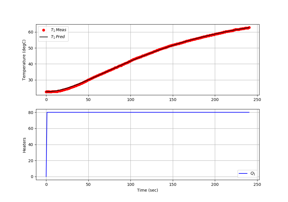
- Item 3: Recorded TCLab data showing measured and predicted temperature responses over the test period.
- Item 4: Plot comparing measured T₁ and predicted T₁ temperatures, showing how parameter estimates evolve during the experiment.
- Item 5: Final identified parameter values (Kₚ, τₛ, ζ) and discussion of how adaptive regression could be applied for PID gain scheduling in nonlinear systems.
- Item 6: Saved figure demonstrating the adaptive parameter fitting process.