Fit Second Order with Optimization
 |  |  |  |
|---|
Fit parameters `K_p` and `\tau_p` from a first order process.
$$G_1(s)=\frac{K_p}{\tau_p \, s + 1}$$
The first order process is in parallel with another first order process.
$$G_2(s)=\frac{-2}{s+1}$$
The combined system has a second order response with data points sampled at 0.5 second intervals from a step input change of 2.0.
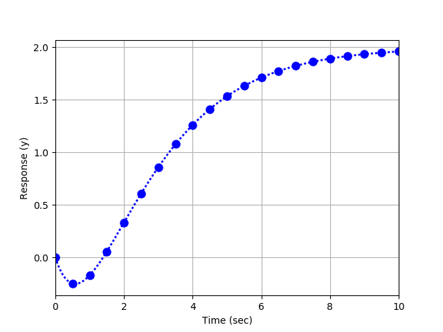

 time, output (y)
 0   , 0
 0.5 , -0.2467
 1   , -0.1677
 1.5 , 0.0583
 2   , 0.3341
 2.5 , 0.6093
 3   , 0.8604
 3.5 , 1.0781
 4   , 1.2613
 4.5 , 1.412
 5   , 1.5344
 5.5 , 1.6328
 6   , 1.7112
 6.5 , 1.7734
 7   , 1.8225
 7.5 , 1.8611
 8   , 1.8914
 8.5 , 1.9152
 9   , 1.9338
 9.5 , 1.9484
 10  , 1.9598
Use optimization to minimize the difference between a predicted response and the 21 measured values. Python and Excel have optimization solvers that may be useful for this exercise.
Scipy Optimize Minimize
import pandas as pd
import matplotlib.pyplot as plt
from scipy.optimize import minimize
# Import data file
# Column 1 = time (t)
# Column 2 = output (ymeas)
url = 'https://apmonitor.com/pdc/uploads/Main/data_2nd_order.txt'
data = pd.read_csv(url)
t = np.array(data['time'])
ymeas = np.array(data['output (y)'])
def model(p):
Kp = p[0]
taup = p[1]
# predicted values
ypred = 2.0 * Kp * (1.0-np.exp(-t/taup)) \
- 4.0 * (1-np.exp(-t))
return ypred
def objective(p):
ypred = model(p)
sse = sum((ymeas-ypred)**2)
return sse
# initial guesses for Kp and taup
p0 = [1.0,1.0]
# show initial objective
print('Initial SSE Objective: ' + str(objective(p0)))
# optimize Kp, taup
solution = minimize(objective,p0)
p = solution.x
# show final objective
print('Final SSE Objective: ' + str(objective(p)))
print('Kp: ' + str(p[0]))
print('taup: ' + str(p[1]))
# calculate new ypred
ypred = model(p)
# plot results
plt.figure()
plt.plot(t,ypred,'r-',linewidth=3,label='Predicted')
plt.plot(t,ymeas,'ko',linewidth=2,label='Measured')
plt.ylabel('Output')
plt.xlabel('Time')
plt.legend(loc='best')
plt.savefig('optimized.png')
plt.show()
GEKKO Optimization Suite
This source code takes a different approach than the Scipy.optimize.minimize or Excel solution where the explicit solution is matched to the data. In this case, the differential equations and the objective function are solved simultaneously. The two first order transfer functions are converted back to differential equation form.
$$\frac{Y_1(s)}{U(s)}=\frac{Kp}{\tau_p s + 1} \rightarrow \tau_p \frac{dy_1}{dt} + y_1 = K_p u$$
$$\frac{Y_2(s)}{U(s)}=\frac{-2}{\tau_p s + 1} \rightarrow \frac{dy_2}{dt} + y_2 = -2 u$$
The two responses `y_1` and `y_2` are computed separately and added together to predict the output `y`.
$$y=y_1+y_2$$
The sum of squared error objective function minimizes the difference between the predicted `y` and the measured `y_{meas}`.
$$\min_{K_p,\tau_p} \left(y-y_{meas}\right)^2$$
import pandas as pd
import matplotlib.pyplot as plt
from gekko import GEKKO
# Import data file
# Column 1 = time (t)
# Column 2 = output (ymeas)
url = 'https://apmonitor.com/pdc/uploads/Main/data_2nd_order.txt'
data = pd.read_csv(url)
t = np.array(data['time'])
ymeas = np.array(data['output (y)'])
# Create GEKKO model
m = GEKKO()
m.time = t
# Inputs
u = 2 # step input
ym = m.Param(ymeas)
# estimate parameters Kp and taup
Kp = m.FV()
taup = m.FV(lb=0)
# turn on parameters (STATUS=1) to let optimize change them
Kp.STATUS = 1
taup.STATUS = 1
# Equation 1
y1 = m.Var(0.0)
m.Equation(taup*y1.dt()==-y1+Kp*u)
# Equation 2
y2 = m.Var(0.0)
m.Equation(y2.dt()+y2==-2*u)
# Summation
y = m.Var(0.0)
m.Equation(y==y1+y2)
# Minimize Objective
m.Obj((y-ym)**2)
# Optimize Kp, taup
m.options.IMODE=5
m.options.NODES=3
m.solve()
# show final objective
print('Final SSE Objective: ' + str(m.options.OBJFCNVAL))
print('Kp: ' + str(Kp.value[0]))
print('taup: ' + str(taup.value[0]))
# plot results
plt.figure()
plt.plot(t,y.value,'r-',linewidth=3,label='Predicted')
plt.plot(t,ymeas,'ko',linewidth=2,label='Measured')
plt.ylabel('Output')
plt.xlabel('Time')
plt.legend(loc='best')
plt.savefig('optimized.png')
plt.show()
What to Turn In
- Item 1: Optimization setup including model equations for G₁(s) and G₂(s) and the combined predicted response equation.
- Item 2: Python or Excel implementation that performs parameter estimation for Kₚ and τₚ by minimizing the sum of squared errors.
- Item 3: Final optimized values of Kₚ and τₚ, and the minimized objective (SSE).
- Item 4: Plot comparing the measured data and the optimized model prediction.
- Item 5: Short discussion explaining which optimization approach was used (e.g., SciPy minimize, GEKKO, or Excel Solver) and how well the model fits the data.