Dynamics and Control

A second-order linear system is a common description of many dynamic processes. The response depends on whether it is an overdamped, critically damped, or underdamped second order system.

$$\tau_s^2 \frac{d^2y}{dt^2} + 2 \zeta \tau_s \frac{dy}{dt} + y = K_p \, u\left(t-\theta_p \right)$$

has output y(t) and input u(t) and four unknown parameters. The four parameters are the gain `K_p`, damping factor `\zeta`, second order time constant `\tau_s`, and dead time `\theta_p`.

Laplace Domain, Transfer Function

In the Laplace domain, the second order system is a transfer function:

$$\frac{Y(s)}{U(s)} = \frac{K_p}{\tau_s^2 s^2 + 2 \zeta \tau_s s + 1}e^{-\theta_p s}$$

State Space Form

To put the second order equation into state space form, it is split into two first order differential equations.

$$\frac{dx_1}{dt} = x_2$$

$$\tau_s^2 \frac{dx_2}{dt} = -2 \zeta \tau_s x_2 - x_1 + K_p u\left(t-\theta_p\right)$$

State `x_1` is the output in state space form.

$$\begin{bmatrix}\dot x_1\\\dot x_2\end{bmatrix} = \begin{bmatrix}0&1\\-\frac{1}{\tau_s^2}&-\frac{2 \zeta}{\tau_s}\end{bmatrix} \begin{bmatrix}x_1\\x_2\end{bmatrix} + \begin{bmatrix}0\\\frac{K_p}{\tau_{s}^2}\end{bmatrix} u\left(t-\theta_p\right)$$

$$y = \begin{bmatrix}1 & 0\end{bmatrix} \begin{bmatrix}x_1\\x_2\end{bmatrix} + \begin{bmatrix}0\end{bmatrix} u$$

Process Gain, `K_p`

The process gain is the change in the output y induced by a unit change in the input u. The process gain is calculated by evaluating the change in y(t) divided by the change in u(t) at steady state initial and final conditions.

$$K_p = \frac{\Delta y}{\Delta u} = \frac{y_{ss_2}-y_{ss_1}}{u_{ss_2}-u_{ss_1}}$$

The process gain affects the magnitude of the response, regardless of the speed of response.

Damping Factor

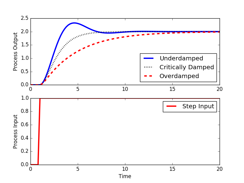
The response of the second order system to a step input in `u(t)` depends whether the system is overdamped `(\zeta>1)`, critically damped `(\zeta=1)`, or underdamped `(0 \le \zeta < 1)`.

1. Overdamped

If the system is overdamped `(\zeta>1)`, the analytic solution to the step response of magnitude M is

$$y(t) = K_p M \left( 1-e^{-\zeta\,t/\tau_s} \left[ \cosh\left( \frac{t}{\tau_s}\sqrt{\zeta^2 - 1} \right) + \frac{\zeta}{\sqrt{\zeta^2-1}} \sinh\left( \frac{t}{\tau_s}\sqrt{\zeta^2 - 1} \right) \right] \right)$$

2. Critically Damped

If the system is critically damped `(\zeta=1)`, the analytic solution to the step response of magnitude M is

$$y(t) = K_p M \left[ 1 - \left( 1+\frac{t}{\tau_s} \right) e^{-t/\tau_s} \right] $$

3. Underdamped (oscillations)

Finally, if the system is underdamped `(0\le\zeta<1)`, the analytic solution to the step response of magnitude M is

$$y(t) = K_p M \left( 1-e^{-\zeta\,t/\tau_s} \left[ \cos\left( \frac{t}{\tau_s}\sqrt{1-\zeta^2} \right) + \frac{\zeta}{\sqrt{1-\zeta^2}} \sin\left( \frac{t}{\tau_s}\sqrt{1-\zeta^2} \right) \right] \right)$$

Second Order Time Constant, `\tau_s`

The second order process time constant is the speed that the output response reaches a new steady state condition. An overdamped second order system may be the combination of two first order systems.

$$\tau_{p1} \frac{dx}{dt} = -x + K_p u \quad \quad \frac{X(s)}{U(s)}=\frac{K_p}{\tau_{p1}\,s + 1}$$

$$\tau_{p2} \frac{dy}{dt} = -y + x \quad \quad \frac{Y(s)}{X(s)}=\frac{1}{\tau_{p2}\,s + 1}$$

The combination of these two first order systems becomes $$\frac{Y(s)}{X(s)}\frac{X(s)}{U(s)}=\frac{Y(s)}{U(s)}=\\\left(\frac{K_p}{\tau_{p1}\,s + 1}\right) \left(\frac{1}{\tau_{p2}\,s + 1}\right) = \frac{K_p}{\tau_{p1}\tau_{p2}\,s^2 + \left(\tau_{p1}+\tau_{p2}\right)s + 1}$$

with `\tau_{p1}\tau_{p2} = \tau_s^2` and `\tau_{p1}+\tau_{p2} = 2 \zeta \tau_s` in second order form.

Process Time Delay, `\theta_p`

The time delay is expressed as a time shift in the input variable u(t).

$$u\left(t-\theta_p\right)$$

The effect of `\theta_p` is to delay the effect of `u(t)`. If `u(t)` is a unit step input that starts at `t=0` then `u(t-\theta_p)` would be a step input that shifts from 0 to 1 at `t=\theta_p`. A time delay adds `e^{-\theta_p \,s }` to the second order transfer function. In the time domain, it replaces any variable `t` with `t-\theta_p` and the output response is multiplied by the step function `S(t-\theta_p)`.

Fit Second Order Model to Data

Two popular methods to fit data or more complex models to a second order system is with a graphical method and step data or with optimization techniques.

• Graphical Method: Fit Second Order Model
• Optimization Method: Fit Second Order Model

Simulate Second Order System