Dynamics and Control

Differential equations are solved in Python with the GEKKO Optimization Suite package.

Jupyter Notebook Gekko Examples on GitHub

Jupyter Notebook GEKKO Examples in Google Colab

GEKKO is available with pip install.

 pip install gekko

GEKKO is an optimization and simulation environment for Python that is different than packages such as Scipy.integrate.ODEINT. In addition to simulation, GEKKO is an optimization platform for dynamic systems.

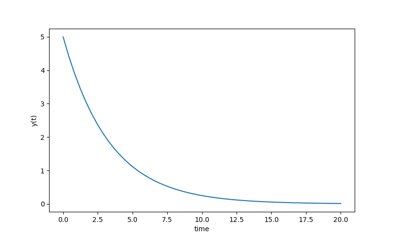
An example of using GEKKO is with the following differential equation with parameter k=0.3, the initial condition y₀=5 and the following differential equation.

$$\frac{dy(t)}{dt} = -k \; y(t)$$

The Python code first imports the needed Numpy, GEKKO, and Matplotlib packages. The model, initial conditions, and time points are defined in GEKKO to numerically calculate y(t).

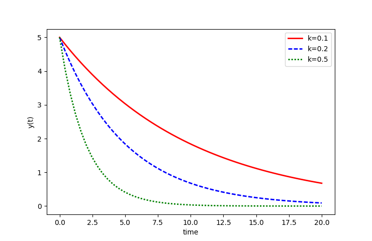
Input parameters such as k can be changed to generate a different solution with a different input parameter. The argument k is now an adjustable parameter.

Exercises

Find a numerical solution to the following differential equations with the associated initial conditions. Expand the requested time horizon until the solution reaches a steady state. Show a plot of the states (x(t) and/or y(t)). Report the final value of each state as `t \to \infty`.

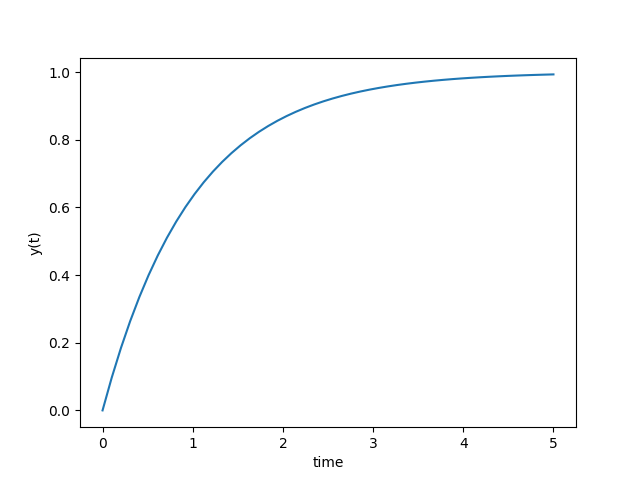
Problem 1

$$\frac{dy(t)}{dt} = -y(t) + 1$$

$$y(0) = 0$$

import numpy as np
from gekko import GEKKO
import matplotlib.pyplot as plt

m = GEKKO()    # create GEKKO model
y = m.Var(0.0) # create GEKKO variable
m.Equation(y.dt()==-y+1) # create GEKKO equation
m.time = np.linspace(0,5) # time points

# solve ODE
m.options.IMODE = 4
m.solve()

# plot results
plt.plot(m.time,y)
plt.xlabel('time')
plt.ylabel('y(t)')

# calculate Steady State
m.options.IMODE = 3
m.solve(disp=False)
print('Final Value: ' + str(y.value))

plt.show()

[$[Get Code]]

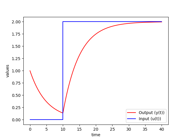
Problem 2

$$5 \; \frac{dy(t)}{dt} = -y(t) + u(t)$$

$$y(0) = 1$$

`u` steps from 0 to 2 at `t=10`

import numpy as np
from gekko import GEKKO
import matplotlib.pyplot as plt

m = GEKKO()    # create GEKKO model
m.time = np.linspace(0,40,401) # time points

# create GEKKO parameter (step 0 to 2 at t=10)
u_step = np.zeros(401)
u_step[100:] = 2.0
u = m.Param(value=u_step)  

y = m.Var(1.0) # create GEKKO variable
m.Equation(5 * y.dt()==-y+u) # create GEKKO equation

# solve ODE
m.options.IMODE = 4
m.solve(disp=False)

# plot results
plt.plot(m.time,y,'r-',label='Output (y(t))')
plt.plot(m.time,u,'b-',label='Input (u(t))')
plt.ylabel('values')
plt.xlabel('time')
plt.legend(loc='best')
plt.show()

[$[Get Code]]

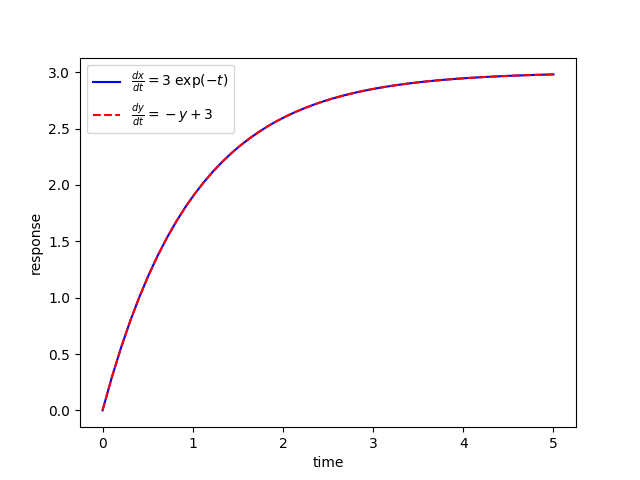
Problem 3

Solve for `x(t)` and `y(t)` and show that the solutions are equivalent.

$$\frac{dx(t)}{dt} = 3 \; exp(-t)$$ $$\frac{dy(t)}{dt} = 3 - y(t)$$ $$x(0) = 0$$ $$y(0) = 0$$

import numpy as np
from gekko import GEKKO
import matplotlib.pyplot as plt

m = GEKKO()    # create GEKKO model
m.time = np.linspace(0,5) # time points

t = m.Var(0.0) # create GEKKO time
x = m.Var(0.0) # create GEKKO variable x
y = m.Var(0.0) # create GEKKO variable y

# create GEKKO equations
m.Equation(t.dt()==1)
m.Equation(x.dt()==3*m.exp(-t))
m.Equation(y.dt()==3-y)

# solve ODE
m.options.IMODE = 4
m.options.NODES = 3
m.solve(disp=False)

# plot results
plt.plot(t,x,'b-',label=r'$\frac{dx}{dt}=3 \; \exp(-t)$')
plt.plot(t,y,'r--',label=r'$\frac{dy}{dt}=-y+3$')
plt.ylabel('response')
plt.xlabel('time')
plt.legend(loc='best')
plt.show()

[$[Get Code]]

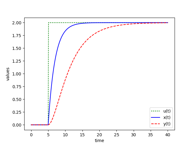
Problem 4

$$2 \; \frac{dx(t)}{dt} = -x(t) + u(t)$$

$$5 \; \frac{dy(t)}{dt} = -y(t) + x(t)$$

$$u = 2 \, S(t-5), \; x(0) = 0, \; y(0) = 0$$

where `S(t-5)` is a step function that changes from zero to one at `t=5`. When it is multiplied by two, it changes from zero to two at that same time, `t=5`.

import numpy as np
from gekko import GEKKO
import matplotlib.pyplot as plt

m = GEKKO()    # create GEKKO model
m.time = np.linspace(0,40,401) # time points

# create GEKKO parameter (step 0 to 2 at t=5)
u_step = np.zeros(401)
u_step[50:] = 2.0
u = m.Param(value=u_step)

# create GEKKO variables
x = m.Var(0.0)
y = m.Var(0.0)

# create GEKKO equations
m.Equation(2*x.dt()==-x+u)
m.Equation(5*y.dt()==-y+x)

# solve ODE
m.options.IMODE = 4
m.solve(disp=False)

# plot results
plt.plot(m.time,u,'g:',label='u(t)')
plt.plot(m.time,x,'b-',label='x(t)')
plt.plot(m.time,y,'r--',label='y(t)')
plt.ylabel('values')
plt.xlabel('time')
plt.legend(loc='best')
plt.show()

[$[Get Code]]

Another Python package that solves differential equations is ODEINT. See this link for the same tutorial with ODEINT versus GEKKO.