Dynamics and Control

Transfer functions are input to output representations of dynamic systems. One advantage of working in the Laplace domain (versus the time domain) is that differential equations become algebraic equations. These algebraic equations can be rearranged and transformed back into the time domain to obtain a solution or further combined with other transfer functions to create more complicated systems. The first step in creating a transfer function is to convert each term of a differential equation with a Laplace transform as shown in the table of Laplace transforms. A transfer function, G(s), relates an input, U(s), to an output, Y(s).

$$G(s) = \frac{Y(s)}{U(s)}$$

First-order Transfer Function

A first-order linear differential equation is shown as a function of time.

$$\tau_p \frac{dy(t)}{dt} = -y(t) + K_p u\left(t-\theta_p\right)$$

The first step is to apply the Laplace transform to each of the terms in the differential equation.

$$\mathcal{L}\left(\tau_p \frac{dy(t)}{dt}\right) = \mathcal{L}\left(-y(t)\right) + \mathcal{L}\left(K_p u\left(t-\theta_p\right)\right)$$

Because the Laplace transform is a linear operator, each term can be transformed separately. With a zero initial condition the value of y is zero at the initial time or y(0)=0.

$$\mathcal{L}\left(\tau_p \frac{dy(t)}{dt}\right) = \tau_p \left(s \, Y(s) - y(0)\right) = \tau_p s \, Y(s)$$

$$\mathcal{L}\left(-y(t)\right) = -Y(s)$$

$$\mathcal{L}\left(K_p u\left(t-\theta_p\right)\right) = K_p \, U(s) \, e^{-\theta_p s}$$

Putting these terms together gives the first-order differential equation in the Laplace domain.

$$\tau_p s \, Y(s) = -Y(s) + K_p \, U(s) \, e^{-\theta_p s}$$

For the first-order linear system, the transfer function is created by isolating terms with Y(s) on the left side of the equation and the term with U(s) on the right side of the equation.

$$\tau_p s \, Y(s) + Y(s) = K_p \, U(s) \, e^{-\theta_p s}$$

Factoring out the Y(s) and dividing through gives the final transfer function.

$$G(s) = \frac{Y(s)}{U(s)} = \frac{K_p e^{-\theta_p s}}{\tau_p s + 1}$$

Transfer Function Gain

The Final Value Theorem (FVT) gives the steady state gain `K_p` of a transfer function `G(s)` by taking the limit as `s \to 0`

$$K_p = \lim_{s \to 0}G(s)$$

This is related to the final value theorem by considering the output response `Y(s)` when the input is a unit step `U(s)=1/s`.

$$K_p = \frac{\Delta y}{\Delta u} = \lim_{s \to 0}G(s) = \lim_{s \to 0}\frac{Y(s)}{U(s)} = \lim_{s \to 0}\frac{Y(s)}{\frac{1}{s}}$$

$$\frac{\Delta y}{\Delta u} = \lim_{s \to 0}\frac{Y(s)}{\frac{1}{s}}$$

In deviation variable form, the initial condition for `u` and `y` is zero.

$$\frac{y_\infty-0}{1-0} = y_\infty = \lim_{s \to 0}\frac{Y(s)}{\frac{1}{s}} = \lim_{s \to 0}s Y(s)$$

The FVT also determines the final signal value `y_\infty` for a stable system with output `Y(s)`. The Laplace variable `s` is multiplied by the signal `Y(s)` before the limit is taken, unlike when calculating the gain.

$$y_\infty = \lim_{s \to 0} s \, Y(s)$$

The FVT may give misleading results if applied to an unstable system. It is only applicable to stable systems. There is additional information on how to determine if a system is stable.

PID Equation in Laplace Domain

The PID equation is a block in an overall control loop diagram.

$$u(t) = u_{bias} + K_c \, e(t) + \frac{K_c}{\tau_I}\int_0^t e(t)dt - K_c \tau_D \frac{d(PV)}{dt}$$

The PID equation can be converted to a transfer function by performing a Laplace transform on each of the elements. The controller output u(t) is combined with the u_bias to create a deviation variable u'(t) = u(t)-u_bias.

$$U(s) = K_c \, E(s) + \frac{K_c}{\tau_I \, s}E(s) - K_c \, \tau_D PV(s)$$

If `\tau_D`=0 for a PI controller, the transfer function for the controller is simplified.

$$G_c(s) = \frac{U(s)}{E(s)} = K_c + \frac{K_c}{\tau_I \, s} = K_c \, \frac{\left(\tau_I s + 1\right)}{\tau_I s}$$

Combining Transfer Functions

The additive property is used for transfer functions in parallel. The input signal `X_1(s)` becomes `Y_1(s)` when it is transformed by `G_1(s)`. Likewise, `X_2(s)` becomes `Y_2(s)` when it is transformed by `G_2(s)`. The two signals `Y_1(s)` and `Y_2(s)` are added to create the final output signal `Y(s)=Y_1(s)+Y_2(s)`. This gives a final output expression of `Y(s)=G_1(s) X_1(s)+G_2(s) X_2(s)`.

The multiplicative property is used for transfer functions in series. The input signal `X_1(s)` becomes `X_2(s)` when it is transformed by `G_1(s)`. The intermediate signal `X_2(s)` becomes the input for the second transfer function `G_2(s)` to produce `Y(s)`. The final output signal is `Y(s)=G_2(s) X_2(s) = G_1(s) G_2(s) X_1(s)`.

Transfer Functions with Python

Python SymPy computes symbolic solutions to many mathematical problems including Laplace transforms. A symbolic and numeric solution is created with the following example problem.

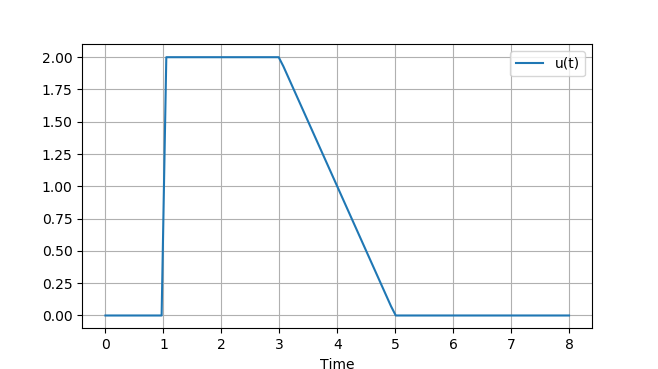
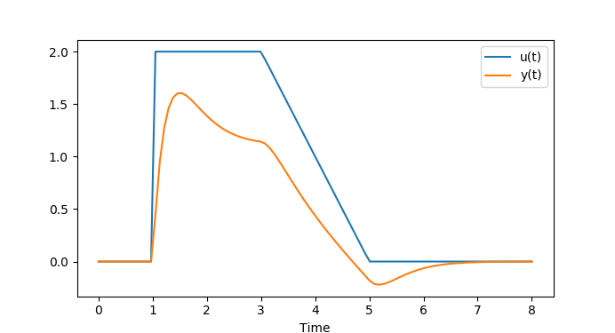
Compute the analytic and numeric system response to an input that includes a step and ramp function.

The system transfer function is a stable system with two poles (denominator roots) and one zero (numerator root):

$$G(s)=\frac{5\left(s + 1\right)}{\left(s + 3\right)^2}$$

Symbolic Solution (Python Sympy)

As a first step, create the step and ramp signals as three individual functions. Compute the system response to each of those three inputs and then sum the signals.

Numeric Solution (Python GEKKO)

An alternative to a symbolic solution is to numerically compute the response in the time domain. The transfer function must first be translated into a differential equation.

$$G(s)=\frac{Y(s)}{U(s)}=\frac{5\left(s + 1\right)}{\left(s + 3\right)^2}$$

$$Y(s)\left(s + 3\right)^2=5\left(s + 1\right)U(s)$$

$$Y(s)\left(s^2 +6s+9\right)=\left(5s + 5\right)U(s)$$

$$\frac{dy^2(t)}{dt^2}+6\frac{dy(t)}{dt}+9y(t)=5\frac{du(t)}{dt}+5u(t)$$

There is additional information on solving differential equations with Python GEKKO or with Python Scipy ODEINT.

Solution (Symbolic and Numeric)

The same solution is found with a analytic or numeric approach.

The advantage of an symbolic (analytic) solution is that it is highly accurate and does not rely on numerical methods to approximate the solution. Also, the solution is in a compact form that can be used for further analysis. Symbolic solutions are limited to cases where the input function and system transfer function can be expressed in Laplace form. This may not be the case for inputs that come from data sources where there the input function has random variation. A symbolic solution with Laplace transforms is also not possible for systems that are nonlinear or complex while numeric solvers can handle many thousands or millions of equations with nonlinear relationships. The disadvantage of a numeric solution is that it is an approximation of the true solution with possible inaccuracies. Another disadvantage is that solvers may fail to converge although this is not typical on problems with an analytic solution.

Assignment

See Transfer Function Exercises