Graphical Method: FOPDT to Step Test
 |  | |  |  |  |
|---|
A first-order linear system with time delay is a common empirical description of many stable dynamic processes. The equation
$$\tau_p \frac{dy(t)}{dt} = -y(t) + K_p u\left(t-\theta_p\right)$$
has variables y(t) and u(t) and three unknown parameters.
$$K_p \quad \mathrm{= Process \; gain}$$
$$\tau_p \quad \mathrm{= Process \; time \; constant}$$
$$\theta_p \quad \mathrm{= Process \; dead \; time}$$
Step test data are convenient for identifying an FOPDT model through a graphical fitting method. Follow the following steps when fitting the parameters `K_p, \tau_p, \theta_p` to a step response.
- Find `\Delta y` from step response
- Find `\Delta u` from step response
- Calculate `K_p = {\Delta y} / {\Delta u}`
- Find `\theta_p`, apparent dead time, from step response
- Find `0.632 \Delta y` from step response
- Find `t_{0.632}` for `y(t_{0.632}) = 0.632 \Delta y` from step response
- Calculate `\tau_p = t_{0.632} - \theta_p`. This assumes that the step starts at `t=0`. If the step happens later, subtract the step time as well.
Exercise
The model below is not a good fit of the process because the parameters have not been adjusted to match the data.
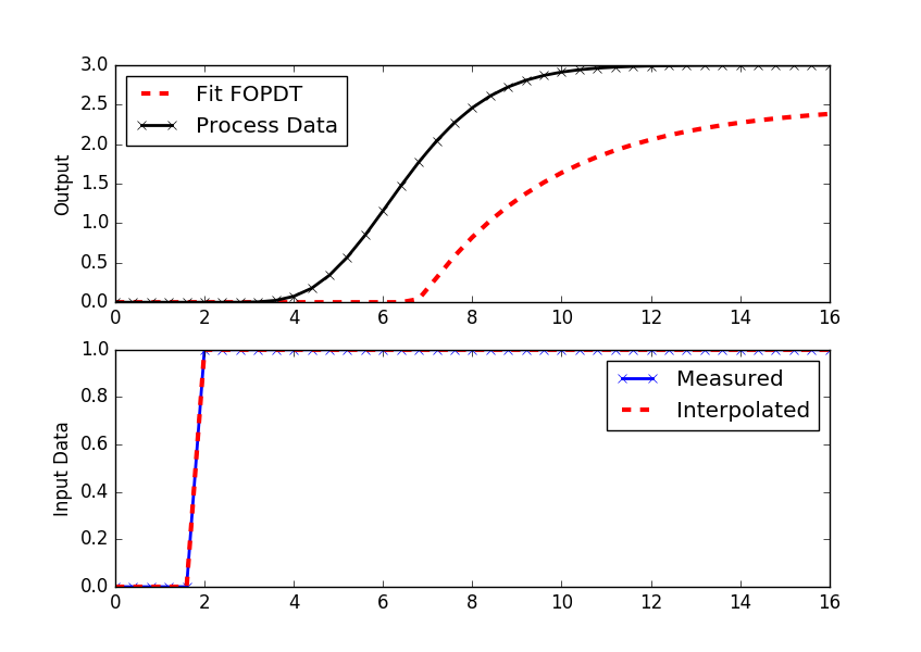
Use the above steps to find parameters `K_p`, `tau_p`, and `\theta_p`. Insert the updated parameters in the code and rerun the script to observe quality of the graphical fit in agreement with the simulated process data.
Km = 2.5
taum = 3.0
thetam = 5.0
ym = sim_model(Km,taum,thetam)
The full code for running the simulation is below. Change only the parameters highlighted above.
import matplotlib.pyplot as plt
from scipy.integrate import odeint
from scipy.optimize import minimize
from scipy.interpolate import interp1d
# define process model (to generate process data)
def process(y,t,n,u,Kp,taup):
# arguments
# y[n] = outputs
# t = time
# n = order of the system
# u = input value
# Kp = process gain
# taup = process time constant
# equations for higher order system
dydt = np.zeros(n)
# calculate derivative
dydt[0] = (-y[0] + Kp * u)/(taup/n)
for i in range(1,n):
dydt[i] = (-y[i] + y[i-1])/(taup/n)
return dydt
# define first-order plus dead-time approximation
def fopdt(y,t,uf,Km,taum,thetam):
# arguments
# y = output
# t = time
# uf = input linear function (for time shift)
# Km = model gain
# taum = model time constant
# thetam = model time constant
# time-shift u
try:
if (t-thetam) <= 0:
um = uf(0.0)
else:
um = uf(t-thetam)
except:
#print('Error with time extrapolation: ' + str(t))
um = 0
# calculate derivative
dydt = (-y + Km * um)/taum
return dydt
# specify number of steps
ns = 40
# define time points
t = np.linspace(0,16,ns+1)
delta_t = t[1]-t[0]
# define input vector
u = np.zeros(ns+1)
u[5:] = 1.0
# create linear interpolation of the u data versus time
uf = interp1d(t,u)
# use this function or replace yp with real process data
def sim_process_data():
# higher order process
n=10 # order
Kp=3.0 # gain
taup=5.0 # time constant
# storage for predictions or data
yp = np.zeros(ns+1) # process
for i in range(1,ns+1):
if i==1:
yp0 = np.zeros(n)
ts = [delta_t*(i-1),delta_t*i]
y = odeint(process,yp0,ts,args=(n,u[i],Kp,taup))
yp0 = y[-1]
yp[i] = y[1][n-1]
return yp
yp = sim_process_data()
# simulate FOPDT model with x=[Km,taum,thetam]
def sim_model(Km,taum,thetam):
# input arguments
#Km
#taum
#thetam
# storage for model values
ym = np.zeros(ns+1) # model
# initial condition
ym[0] = 0
# loop through time steps
for i in range(1,ns+1):
ts = [delta_t*(i-1),delta_t*i]
y1 = odeint(fopdt,ym[i-1],ts,args=(uf,Km,taum,thetam))
ym[i] = y1[-1]
return ym
# calculate model with updated parameters
Km = 2.5
taum = 3.0
thetam = 5.0
ym = sim_model(Km,taum,thetam)
# plot results
plt.figure()
plt.subplot(2,1,1)
plt.plot(t,ym,'r--',linewidth=3,label='Fit FOPDT')
plt.plot(t,yp,'kx-',linewidth=2,label='Process Data')
plt.ylabel('Output')
plt.legend(loc='best')
plt.subplot(2,1,2)
plt.plot(t,u,'bx-',linewidth=2)
plt.plot(t,uf(t),'r--',linewidth=3)
plt.legend(['Measured','Interpolated'],loc='best')
plt.ylabel('Input Data')
plt.show()
Self-Assessment
Test your knowledge on First Order Graphical Fit