Quiz: FOPDT Graphical Fit
 |  | | |  |  |
|---|
Learn: First-Order Linear Dynamics with Dead Time using Graphical Fitting Methods
1. One time constant is the amount of time to get to `1-e^{-1}=0.632` or 63.2% of the way to steady state from 0 to 1. It comes from the analytic solution of the first order differential equation `\tau \frac{dy}{dt} + y = u` with `u=1`.
$$y(t)=\left( 1 - e^{-t / \tau} \right)$$
What is the value of `y(t)` at two time constants `t=2\tau`?
- Incorrect. This is the value of `y(t)` at one time constant where `y(3\tau)=( 1 - e^{-1})=0.632`.
- Incorrect. This is the value of `y(t)` at three time constants where `y(3\tau)=( 1 - e^{-3})=0.95`.
- Correct. This is the value of `y(t)` at two time constants where `y(2\tau)=( 1 - e^{-2})=0.86`.
- Incorrect. This is the value of `y(t)` at five time constants where `y(5\tau)=( 1 - e^{-5})=0.993`.
Use this information to answer questions 2-4. A first-order linear system with time delay is a common empirical description of many stable dynamic processes. The equation
$$\tau_p \frac{dy(t)}{dt} = -y(t) + K_p u\left(t-\theta_p\right)$$
has variables y(t) and u(t) and three unknown parameters.
$$K_p \quad \mathrm{= Process \; gain}$$
$$\tau_p \quad \mathrm{= Process \; time \; constant}$$
$$\theta_p \quad \mathrm{= Process \; dead \; time}$$
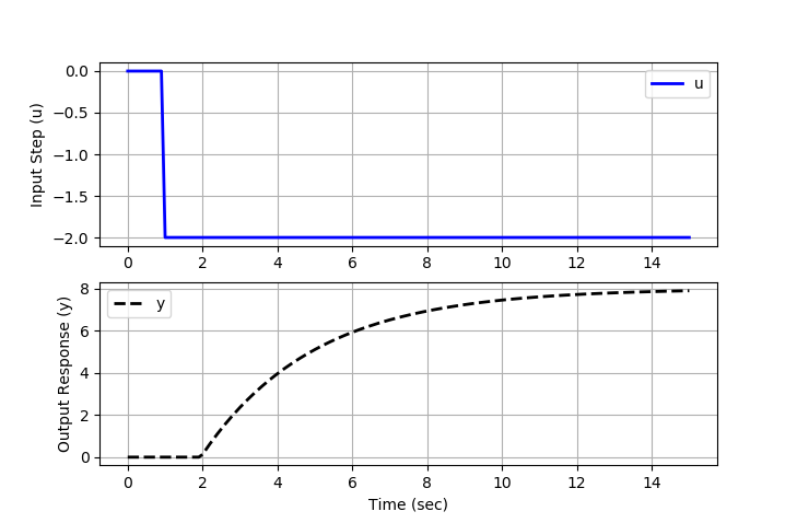
2. Determine the value of `K_p` that best fits the step response data.
- Correct. The gain is `K_p = \frac{\Delta y}{\Delta u} = \frac{8}{-2} = -4`.
- Incorrect. This answer is the change `\Delta y=8`. The gain is `K_p = \frac{\Delta y}{\Delta u}`. Don't forget to divide by the input step `\Delta u=-2`
- Incorrect. The gain is negative because a decrease in the input leads to an increase in the response. An increase in the input will likewise lead to a decrease in the response.
- Incorrect. You may be confusing gain with time delay.
3. Determine the value of `\theta_p` that best fits the step response data.
- Incorrect. The input step starts at 1 sec, not 0 sec. The time delay is the difference between the time when the output response starts to respond and the input step time.
- Correct. The time delay `\theta_p=2-1=1` is the difference between the time when the output response starts to respond (t=2) and the input step time (t=1).
- Incorrect. The time delay is always `\ge 0`.
- Incorrect. Time units are important. The plot is in seconds.
4. Determine the value of `\tau_p` that best fits the step response data.
- Incorrect. You may be confusing time constant `\tau_p` with time delay `\theta_p`.
- Incorrect. The time constant is always `\ge 0`.
- Incorrect. The time to reach 63.2% of the response does not include the time delay. Shift to account for the time delay before calculating the time constant.
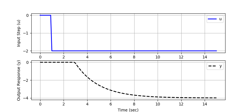
- Correct. You can check the step response with the Python code below.
You can test your FOPDT parameters with the Python script. Update the values of Km, taum, and thetam and run the program.
Km = 2.0
taum = 2.0
thetam = 2.0
import matplotlib.pyplot as plt
from scipy.integrate import odeint
from scipy.interpolate import interp1d
# define first-order plus dead-time approximation
def fopdt(y,t,uf,Km,taum,thetam):
# arguments
# y = output
# t = time
# uf = input linear function (for time shift)
# Km = model gain
# taum = model time constant
# thetam = model time constant
# time-shift u
try:
if (t-thetam) <= 0:
um = uf(0.0)
else:
um = uf(t-thetam)
except:
um = 0
# calculate derivative
dydt = (-y + Km * um)/taum
return dydt
# specify number of steps
ns = 150
# define time points
t = np.linspace(0,15,ns+1)
delta_t = t[1]-t[0]
# define input vector
u = np.zeros(ns+1)
u[10:] = -2.0
# create linear interpolation of the u data versus time
uf = interp1d(t,u)
# simulate FOPDT model with x=[Km,taum,thetam]
def sim_model(Km,taum,thetam):
# input arguments
#Km
#taum
#thetam
# storage for model values
ym = np.zeros(ns+1) # model
# initial condition
ym[0] = 0
# loop through time steps
for i in range(1,ns+1):
ts = [delta_t*(i-1),delta_t*i]
y1 = odeint(fopdt,ym[i-1],ts,args=(uf,Km,taum,thetam))
ym[i] = y1[-1]
return ym
# calculate model with updated parameters
Km = 2.0
taum = 2.0
thetam = 2.0
ym = sim_model(Km,taum,thetam)
# plot results
plt.figure()
plt.subplot(2,1,1)
plt.plot(t,u,'b-',linewidth=2)
plt.legend(['u'],loc='best')
plt.ylabel('Input Step (u)')
plt.grid()
plt.subplot(2,1,2)
plt.plot(t,ym,'k--',linewidth=2,label='y')
plt.ylabel('Output Response (y)')
plt.legend(loc='best')
plt.xlabel('Time (sec)')
plt.grid()
plt.show()