State Space Models
 |  |  |  |
|---|
Linear Time Invariant (LTI) state space models are a linear representation of a dynamic system in either discrete or continuous time. Putting a model into state space form is the basis for many methods in process dynamics and control analysis. Below is the continuous time form of a model in state space form.
$$\dot x = A x + B u$$
$$y = C x + D u$$
with states `x in \mathbb{R}^n` and state derivatives `\dot x = {dx}/{dt} in \mathbb{R}^n`. The notation `in \mathbb{R}^n` means that `x` and `\dot x` are in the set of real-numbered vectors of length `n`. The other elements are the outputs `y in \mathbb{R}^p`, the inputs `u in \mathbb{R}^m`, the state transition matrix `A`, the input matrix `B`, and the output matrix `C`. The remaining matrix `D` is typically zeros because the inputs do not typically affect the outputs directly. The dimensions of each matrix are shown below with `m` inputs, `n` states, and `p` outputs.
$$A \in \mathbb{R}^{n \, \mathrm{x} \, n}$$ $$B \in \mathbb{R}^{n \, \mathrm{x} \, m}$$ $$C \in \mathbb{R}^{p \, \mathrm{x} \, n}$$ $$D \in \mathbb{R}^{p \, \mathrm{x} \, m}$$
Stability
The linear state space model is stable if all eigenvalues of A are negative real numbers or have negative real parts to complex number eigenvalues. If all real parts of the eigenvalues are negative then the system is stable, meaning that any initial condition converges exponentially to a stable attracting point. If any real parts are zero then the system will not converge to a point and if the eigenvalues are positive the system is unstable and will exponentially diverge.
First Order System in State Space
The state space form can be difficult to grasp at first so consider an example to transform a first order linear system (without time delay) into state space form.
$$\tau_p \frac{dy}{dt} = -y + K_p u$$
Divide both sides by `\tau_p` and add the output relationship `x = y` and `\dot x = \dot y` to give the following in state space form.
$$\dot x = \left[-\frac{1}{\tau_p}\right] x + \left[\frac{K_p}{\tau_p}\right] u$$
$$y = [1] x + [0] u$$
Second Order System in State Space
A second order linear system has `x in \mathbb{R}^2`, `y in \mathbb{R}^1`, `u in \mathbb{R}^1`, `A in \mathbb{R}^{2x2}`, `B in \mathbb{R}^{2x1}`, `C in \mathbb{R}^{1x2}` and `D in \mathbb{R}^{1x1}`. A second order overdamped system can be expressed as two first order linear systems in series.
$$\tau_{p1} \frac{dx_1}{dt} = -x_1 + K_p u$$
$$\tau_{p2} \frac{dx_2}{dt} = -x_2 + x_1$$
$$y = x_2$$
Dividing by `\tau_{p1}` and `\tau_{p2}` gives the following in state space form.
$$\begin{bmatrix}\dot x_1\\\dot x_2\end{bmatrix} = \begin{bmatrix}-\frac{1}{\tau_{p1}}&0\\\frac{1}{\tau_{p2}}&-\frac{1}{\tau_{p2}}\end{bmatrix} \begin{bmatrix}x_1\\x_2\end{bmatrix} + \begin{bmatrix}\frac{K_p}{\tau_{p1}}\\0\end{bmatrix} u$$
$$y = \begin{bmatrix}0 & 1\end{bmatrix} \begin{bmatrix}x_1\\x_2\end{bmatrix} + \begin{bmatrix}0\end{bmatrix} u$$
General Nonlinear System
Consider a nonlinear differential equation model that is derived from balance equations with input u, states x, and output y.
$$\frac{dx}{dt} = f(x,u)$$
$$y = g(x)$$
The expressions for `f(x,u)` and `g(x)` are linearized by a Taylor series expansion, using only the first two terms as found on the page for model linearization.
$$\frac{dx}{dt} = f(x,u) \approx f \left(\bar x, \bar u\right) + \frac{\partial f}{\partial x}\bigg|_{\bar x,\bar u} \left(x-\bar x\right) + \frac{\partial f}{\partial u}\bigg|_{\bar x,\bar u} \left(u-\bar u\right)$$
$$y-\bar y = g(x) \approx g \left(\bar x\right) + \frac{\partial f}{\partial x}\bigg|_{\bar x} \left(x-\bar x\right)$$
If the values of `\bar u` and `\bar x` are chosen at steady state conditions then `f(\bar x, \bar u)=0` because the derivative term `{dx}/{du}=0` at steady state. To simplify the final linearized expression, deviation variables are defined as `y' = y-\bar y`, `x' = x-\bar x` and `u' = u - \bar u`. A deviation variable is a change from the nominal steady state conditions. The derivatives of the deviation variable are defined as `{dx'}/{dt} = {dx}/{dt}` because `{d\bar x}/{dt} = 0` in `{dx'}/{dt} = {d(x-\bar x)}/{dt} = {dx}/{dt} - \cancel{{d\bar x}/{dt}}`. If there are additional variables such as a disturbance variable `d` then it is added as another input term in deviation variable form.
$$\frac{dx'}{dt} = \alpha \, y' + \beta \, u'$$
$$y' = \gamma \, x'$$
The values of the constants `\alpha` and `\beta` are the partial derivatives of `f(x,u)` and the value of the constant `\gamma` is the partial derivative of `g(x)`, all evaluated as steady state conditions.
$$\alpha = \frac{\partial f}{\partial x}\bigg|_{\bar x,\bar u} \quad \quad \beta = \frac{\partial f}{\partial u}\bigg|_{\bar x,\bar u} \quad \quad \gamma = \frac{\partial g}{\partial x}\bigg|_{\bar x}$$
In cases with more than one `u`, `x`, or `y` the general form of the linearized model in state space form with three inputs, two states, and two outputs is
$$\begin{bmatrix}\dot x_1'\\\dot x_2'\end{bmatrix} = \begin{bmatrix}\frac{\partial f_1}{\partial x_1}\bigg|_{\bar x,\bar u}&\frac{\partial f_1}{\partial x_2}\bigg|_{\bar x,\bar u}\\\frac{\partial f_2}{\partial x_1}\bigg|_{\bar x,\bar u}&\frac{\partial f_2}{\partial x_2}\bigg|_{\bar x,\bar u}\end{bmatrix} \begin{bmatrix}x_1'\\x_2'\end{bmatrix} + \begin{bmatrix}\frac{\partial f_1}{\partial u_1}\bigg|_{\bar x,\bar u}&\frac{\partial f_1}{\partial u_2}\bigg|_{\bar x,\bar u}&\frac{\partial f_1}{\partial u_3}\bigg|_{\bar x,\bar u}\\\frac{\partial f_2}{\partial u_1}\bigg|_{\bar x,\bar u}&\frac{\partial f_2}{\partial u_2}\bigg|_{\bar x,\bar u}&\frac{\partial f_2}{\partial u_3}\bigg|_{\bar x,\bar u} \end{bmatrix} \begin{bmatrix}u_1'\\u_2'\\u_3'\end{bmatrix}$$
$$\begin{bmatrix}y_1'\\y_2'\end{bmatrix} = \begin{bmatrix} \frac{\partial g_1}{\partial x_1}\bigg|_{\bar x}&\frac{\partial g_1}{\partial x_2}\bigg|_{\bar x}\\\frac{\partial g_2}{\partial x_1}\bigg|_{\bar x}&\frac{\partial g_2}{\partial x_2}\bigg|_{\bar x}\end{bmatrix} \begin{bmatrix}x_1'\\x_2'\end{bmatrix}$$
An exercise in linearizing a highly nonlinear model is given as an exercise for State Space Modeling.
Exercise
Put the following equations into state space form by determining matrices A, B, C, and D.
$$\dot x = A x + B u$$ $$y = C x + D u$$
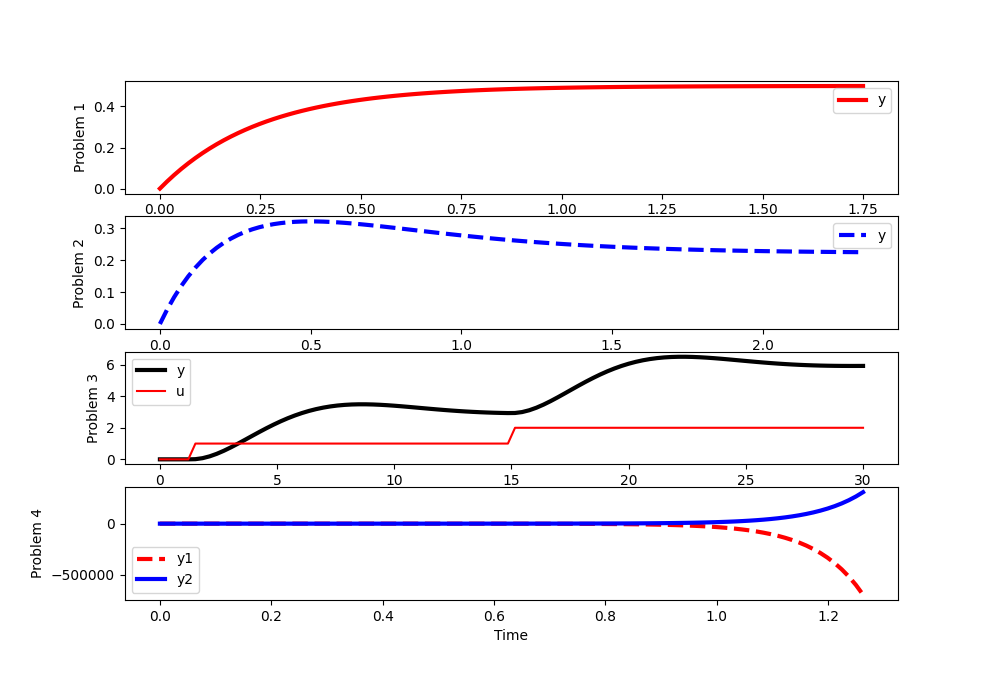
Simulate a step response for each model and determine whether the system is stable or unstable.
1. First order differential equation
$$3 \, \frac{dx}{dt} + 12 \, x = 6 \, u$$ $$y = x$$
2. Second order differential equations
$$2 \frac{dx_1}{dt} + 6 \, x_1 = 8 \, u$$ $$3 \frac{dx_2}{dt} + 6 \, x_1 + 9 \, x_2 = 0$$ $$y = \frac{x_1 + x_2}{2}$$
3. Second order differential equation
$$4 \frac{d^2y}{dt^2} + 2 \frac{dy}{dt} + y = 3 \, u$$
4. Nonlinear differential equations
$$2 \frac{dx_1}{dt} + x_1^2 + 3 \, x_2^2 = 16 \, u$$ $$3 \frac{dx_2}{dt} + 6 \, x_1^2 - 6 \, x_2^2 = 0$$ $$y_1 = x_2$$ $$y_2 = x_1$$
$$\bar u = 1, \quad \bar x = \begin{bmatrix}2\\2\end{bmatrix}$$
Solution
Correction (thanks to Hira Shroff): Changed the second differential equation of Problem 4 from the original form that is not at steady state at the equilibrium point:
$$3 \frac{dx_2}{dt} + 6 \, x_1^2 + 6 \, x_2^2 = 0$$
to the new equation has a negative sign:
$$3 \frac{dx_2}{dt} + 6 \, x_1^2 - 6 \, x_2^2 = 0$$
The solution for Problem 4 in the video is incorrect as it uses the original form. The solution code has been corrected.
from scipy import signal
# problem 1
A = [-4.0]
B = [2.0]
C = [1.0]
D = [0.0]
sys1 = signal.StateSpace(A,B,C,D)
t1,y1 = signal.step(sys1)
# problem 2
A = [[-3.0,0.0],[-2.0,-3.0]]
print(np.linalg.eig(A)[0])
B = [[4.0],[0.0]]
C = [0.5,0.5]
D = [0.0]
sys2 = signal.StateSpace(A,B,C,D)
t2,y2 = signal.step(sys2)
# problem 3
A = [[0.0,1.0],[-0.25,-0.5]]
print(np.linalg.eig(A)[0])
B = [[0.0],[0.75]]
C = [1.0,0.0]
D = [0.0]
sys3 = signal.StateSpace(A,B,C,D)
t = np.linspace(0,30,100)
u = np.zeros(len(t))
u[5:50] = 1.0 # first step input
u[50:] = 2.0 # second step input
t3,y3,x3 = signal.lsim(sys3,u,t)
# problem 4
A = [[-2.0,-6.0],[-8.0,8.0]]
print(np.linalg.eig(A)[0])
B = [[8.0],[0.0]]
C = [[0.0,1.0],[1.0,0.0]]
D = [[0.0],[0.0]]
sys4 = signal.StateSpace(A,B,C,D)
t4,y4 = signal.step(sys4)
import matplotlib.pyplot as plt
plt.figure(1)
plt.subplot(4,1,1)
plt.plot(t1,y1,'r-',linewidth=3)
plt.ylabel('Problem 1')
plt.legend(['y'],loc='best')
plt.subplot(4,1,2)
plt.plot(t2,y2,'b--',linewidth=3)
plt.ylabel('Problem 2')
plt.legend(['y'],loc='best')
plt.subplot(4,1,3)
plt.plot(t3,y3,'k-',linewidth=3)
plt.plot(t,u,'r-')
plt.ylabel('Problem 3')
plt.legend(['y','u'],loc='best')
plt.subplot(4,1,4)
plt.plot(t4,y4[:,0]+2.0,'r--',linewidth=3)
plt.plot(t4,y4[:,1]+2.0,'b-',linewidth=3)
plt.legend(['y1','y2'],loc='best')
plt.ylabel('Problem 4')
plt.xlabel('Time')
plt.show()