Graphically Fit Second Order Response
 |  |  |  |  |
|---|
Oscillating systems need a different type of model than a first order model form for an acceptable approximation. Oscillations imply that the system is an underdamped system. A second order approximation is given by the following equation in the time domain
$$\tau_s^2 \frac{d^2y}{dt^2} + 2 \zeta \tau_s \frac{dy}{dt} + y = K_p \, u\left(t-\theta_p \right)$$
with output y(t), input u(t) and four unknown parameters. The four parameters are the gain `K_p`, damping factor `\zeta`, second order time constant `\tau_s`, and dead time `\theta_p`.
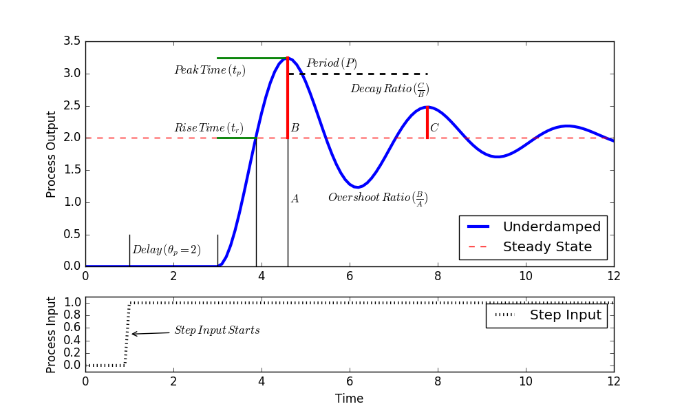
The following are steps to obtain a graphical approximation of a step response of an underdamped (oscillating) second order system. An underdamped system implies that `0 \le \zeta < 1`.
- Find `\Delta y` from step response.
- Find `\Delta u` from step response.
- Calculate `K_p = {\Delta y} / {\Delta u}`.
- Calculate damping factor `\zeta` from overshoot `OS` or decay ratio `DR`.
- Calculate `\tau_s` from equations for rise time `t_r`, peak time `t_p`, or period `P`.
import matplotlib.pyplot as plt
import matplotlib.gridspec as gs
from scipy.integrate import odeint
# specify number of steps
ns = 120
# define time points
t = np.linspace(0,ns/10.0,ns+1)
class model(object):
# default process model
Kp = 2.0
taus = 0.5
thetap = 2.0
zeta = 0.15
def process(x,t,u,Kp,taus,zeta):
# Kp = process gain
# taus = second order time constant
# zeta = damping factor
# ts^2 dy2/dt2 + 2 zeta taus dydt + y = Kp u(t-thetap)
y = x[0]
dydt = x[1]
dy2dt2 = (-2.0*zeta*taus*dydt - y + Kp*u)/taus**2
return [dydt,dy2dt2]
def calc_response(t,m):
# t = time points
# m = process model
Kp = m.Kp
taus = m.taus
thetap = m.thetap
zeta = m.zeta
print('Kp: ' + str(Kp))
print('taus: ' + str(taus))
print('zeta: ' + str(zeta))
# specify number of steps
ns = len(t)-1
delta_t = t[1]-t[0]
# storage for recording values
op = np.zeros(ns+1) # controller output
pv = np.zeros((ns+1,2)) # process variable
# step input
op[10:]=1.0
# Simulate time delay
ndelay = int(np.ceil(thetap / delta_t))
# loop through time steps
for i in range(0,ns):
# implement time delay
iop = max(0,i-ndelay)
inputs = (op[iop],Kp,taus,zeta)
y = odeint(process,pv[i],[0,delta_t],args=inputs)
pv[i+1] = y[-1]
return (pv,op)
# underdamped step response
(pv,op) = calc_response(t,model)
# rename parameters
tau = model.taus
zeta = model.zeta
du = 2.0
s = 3.0
# peak time
tp = np.pi * tau / np.sqrt(1.0-zeta**2)
# rise time
tr = tau / (np.sqrt(1.0-zeta**2)) * (np.pi-np.arccos(zeta))
# overshoot ratio
os = np.exp(-np.pi * zeta / (np.sqrt(1.0-zeta**2)))
# decay ratio
dr = os**2
# period
p = 2.0 * np.pi * tau / (np.sqrt(1.0-zeta**2))
print('Summary of response')
print('rise time: ' + str(tr))
print('peak time: ' + str(tp))
print('overshoot: ' + str(os))
print('decay ratio: ' + str(dr))
print('period: ' + str(p))
plt.figure(1)
g = gs.GridSpec(2, 1, height_ratios=[3, 1])
ap = {'arrowstyle': '->'}
plt.subplot(g[0])
plt.plot(t,pv[:,0],'b-',linewidth=3,label='Underdamped')
plt.plot([0,max(t)],[2.0,2.0],'r--',label='Steady State')
plt.plot([1,1],[0,0.5],'k-')
plt.plot([3,3],[0,0.5],'k-')
plt.plot([3+tr,3+tr],[0,2],'k-')
plt.plot([3+tp,3+tp],[0,2],'k-')
plt.plot([3,3+tr],[2,2],'g-',linewidth=2)
plt.plot([3,3+tp],[2*(1+os),2*(1+os)],'g-',linewidth=2)
plt.plot([3+tp,3+tp+p],[3,3],'k--',linewidth=2)
plt.plot([3+tp,3+tp],[2,2*(1.0+os)],'r-',linewidth=3)
plt.plot([3+tp+p,3+tp+p],[2,2*(1+os*dr)],'r-',linewidth=3)
plt.legend(loc=4)
plt.ylabel('Process Output')
tloc = (1.05,0.2)
txt = r'$Delay\,(\theta_p=2)$'
plt.annotate(s=txt,xy=tloc)
tloc = (2,2.1)
txt = r'$Rise\,Time\,(t_r)$'
plt.annotate(s=txt,xy=tloc)
tloc = (2,3)
txt = r'$Peak\,Time\,(t_p)$'
plt.annotate(s=txt,xy=tloc)
tloc = (5,3.1)
txt = r'$Period\,(P)$'
plt.annotate(s=txt,xy=tloc)
tloc = (3+tp+0.05,1.0)
txt = r'$A$'
plt.annotate(s=txt,xy=tloc)
tloc = (3+tp+0.05,2.1)
txt = r'$B$'
plt.annotate(s=txt,xy=tloc)
tloc = (3+tp+p+0.05,2.1)
txt = r'$C$'
plt.annotate(s=txt,xy=tloc)
tloc = (6,2.7)
txt = r'$Decay\,Ratio\,(\frac{C}{B})$'
plt.annotate(s=txt,xy=tloc)
tloc = (5.5,1.0)
txt = r'$Overshoot\,Ratio\,(\frac{B}{A})$'
plt.annotate(s=txt,xy=tloc)
plt.subplot(g[1])
plt.plot(t,op,'k:',linewidth=3,label='Step Input')
plt.ylim([-0.1,1.1])
plt.legend(loc='best')
plt.ylabel('Process Input')
plt.xlabel('Time')
pt = (1.0,0.5)
tloc = (2.0,0.5)
txt = r'$Step\,Input\,Starts$'
plt.annotate(s=txt,xy=pt,xytext=tloc,arrowprops=ap)
plt.savefig('output.png')
plt.show()
The graphical metrics are dependent on `\zeta` and `\tau_s` with the following correlations. For example, it is easiest to use equations for overshoot and decay ratio to calculate `\zeta`. The value for `\tau_s` can then be calculated from rise time `t_r`, peak time `t_p`, or period `P`.
- Rise time `t_r`: amount of time to first cross the steady state level (after accounting for dead time).
$$t_r = \frac{\tau_s}{\sqrt{1-\zeta^2}}\left( \pi - cos^{-1} \zeta \right)$$
- Peak time `t_p`: amount of time to reach the first peak (after accounting for dead time).
$$t_p = \frac{\pi \tau_s}{\sqrt{1-\zeta^2}} \quad \quad \tau_s = \frac{\sqrt{1-\zeta^2}}{\pi}t_p$$
- Overshoot ratio `OS`: amount that first oscillation surpasses the steady state level relative to the steady state change
$$OS = \exp\left({-\frac{\pi \zeta}{\sqrt{1-\zeta^2}}}\right) \quad \quad \zeta = \sqrt{\frac{\left(\ln(OS)\right)^2}{\pi^2 + \left(\ln(OS)\right)^2}}$$
- Decay ratio `DR`: fractional size of successive peaks
$$DR = OS^2 = \exp\left({-\frac{2 \pi \zeta}{\sqrt{1-\zeta^2}}}\right)$$
- Period `P`: the length of time for an oscillation from peak to peak
$$P = \frac{2 \pi \tau_s}{\sqrt{1-\zeta^2}} \quad \quad \tau_s = \frac{\sqrt{1-\zeta^2}}{2 \pi}P$$
Another method to obtain the parameters is with an optimization method such as minimizing a sum of squared errors differences between measured and predicted values.
Assignment