Dynamics and Control

A PID (Proportional-Integral-Derivative) controller is a control loop feedback mechanism widely used in industrial control systems and other applications requiring continuously modulated control. It is a type of control system that uses feedback to continuously adjust the output of a process or system to match a desired setpoint.

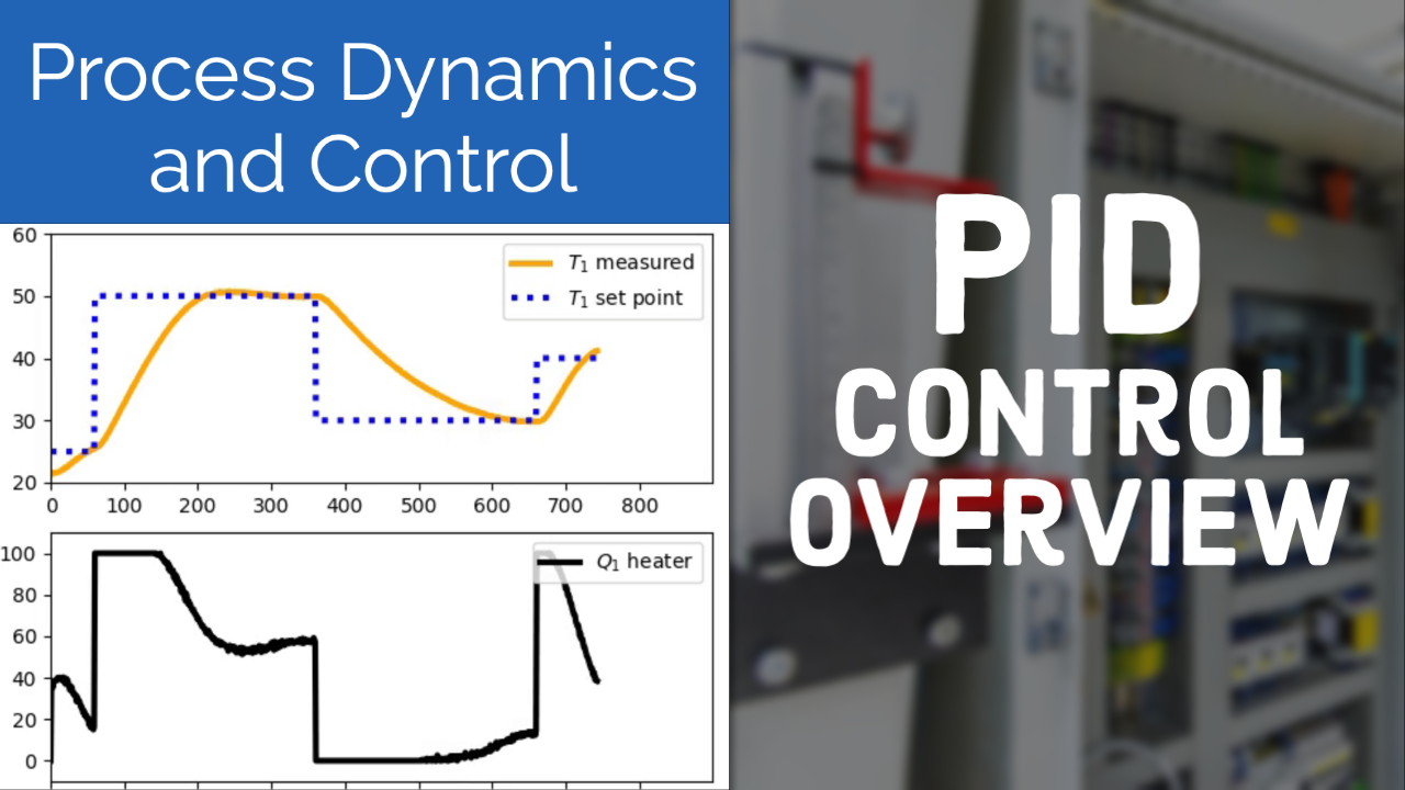
PID controllers are widely used in a variety of applications, including temperature control, flow control, and motor control, due to the PID ability to provide stable and accurate control with relatively simple implementation. Below is an example with the Arduino-based Temperature Control Lab.

A PID (Proportional Integral Derivative) controller consists of three components that are adjusted based on the difference between a set point (SP) and a measured process variable (PV).

$$e(t) = SP-PV$$

The output of a PID controller (u(t)) is calculated using the sum of the Proportional, Integral, and Derivative terms where KP, KI, and KD are constants that can be adjusted to fine-tune the performance of the controller.

$$u(t) = \mathrm{KP}\,\color{red}{e(t)} + \mathrm{KI}\color{green}{\int_0^t e(t)dt} + \mathrm{KD} \color{blue}{\frac{de(t)}{dt}}$$

$$\mathrm{Output = \color{red}{Proportional} + \color{green}{Integral} + \color{blue}{Derivative}}$$

Proportional (P) control: This component adjusts the output of the process based on the current error between the setpoint and the process variable (PV). The larger the error, the larger the correction applied.

$$\mathrm{Proportional} = \mathrm{KP} \, e(t)$$

Integral (I) control: This component adjusts the output based on the accumulated error over time. It helps eliminate steady-state error and can improve the stability of the control system.

$$\mathrm{Integral} = \mathrm{KI}\int_0^t e(t)dt$$

Derivative (D) control: This component adjusts the output based on the rate of change of the error. It helps to dampen oscillations and improve the stability of the control system but is often omitted because PI control is sufficient. The derivative term can amplify measurement noise (random fluctuations) and cause excessive output changes. Filters are important to get a better estimate of the process variable rate of change.

$$\mathrm{Derivative} = \mathrm{KD}\frac{de(t)}{dt} = - \mathrm{KD} \frac{d(PV)}{dt}$$

The derivative of the error is substituted with the derivative of the Process Variable (PV) to avoid derivative kick when there is a setpoint change. The value of the controller output `u(t)` is transferred as the system input. The KP, KI, and KD parameters from the Independent form can also be written in terms of controller gain `K_c`, integral reset time `\tau_I`, and derivative time constant `\tau_D`. All terms depend on a single controller gain `K_c` and this is known as the Dependent form of the PID equation.

$$\mathrm{KP} = K_c, \quad \mathrm{KI} = \frac{K_c}{\tau_I}, \quad \mathrm{KD} = K_c \tau_D$$

$$u(t) = u_{bias} + K_c \, e(t) + \frac{K_c}{\tau_I}\int_0^t e(t)dt - K_c \tau_D \frac{d(PV)}{dt}$$

$$\mathrm{Output = Bias + Proportional + Integral + Derivative}$$

The `u_{bias}` term is a constant that is typically set to the value of `u(t)` when the controller is first switched from manual to automatic mode. This gives bumpless transfer if the error is zero when the controller is turned on. The three tuning values for a PID controller are the controller gain, `K_c`, the integral time constant `\tau_I`, and the derivative time constant `\tau_D`. The value of `K_c` is a multiplier on the proportional error and integral term and a higher value makes the controller more aggressive at responding to errors away from the set point. The integral time constant `\tau_I` (also known as integral reset time) must be positive and has units of time. As `\tau_I` gets smaller, the integral term is larger because `\tau_I` is in the denominator. Derivative time constant `\tau_D` also has units of time and must be positive. The set point (SP) is the target value and process variable (PV) is the measured value that may deviate from the desired value. The error from the set point is the difference between the SP and PV and is defined as `e(t) = SP - PV`.

Overview of PID Control

PI or PID controller is best suited for non-integrating processes, meaning any process that eventually returns to the same output given the same set of inputs and disturbances. A P-only controller is best suited to integrating processes. Integral action is used to remove offset and can be thought of as an adjustable `u_{bias}`.

Discrete PID Controller

Digital controllers are implemented with discrete sampling periods and a discrete form of the PID equation is needed to approximate the integral of the error and the derivative. This modification replaces the continuous form of the integral with a summation of the error and uses `\Delta t` as the time between sampling instances and `k` as the number of sampling instances. It also replaces the derivative with either a filtered version of the derivative or another method to approximate the instantaneous slope of the (PV).

$$u_k = u_{bias} + K_c \, e_k + \frac{K_c}{\tau_I}\sum_{i=1}^{k} e_i\Delta t - K_c \tau_D \frac{PV_k-PV_{k-1}}{\Delta t}$$

The same tuning correlations are used for both the continuous and discrete forms of the PID controller.

PID Velocity Form

An alternative to the positional form shown above is the velocity form. This is commonly implemented in control systems such as Programmable Logic Controllers (PLCs) and Distributed Control Systems (DCSs) for industrial control. The advantage of the velocity form is that changes in the Proportional and Integral tuning parameters do not lead to sudden jumps in the controller output. The velocity form is obtained by differentiating the positional form.

$$\frac{u(t)}{dt} = \mathrm{KP}\,\color{red}{\frac{e(t)}{dt}} + \mathrm{KI}\color{green}{e(t)} + \mathrm{KD} \color{blue}{\frac{d^2e(t)}{dt^2}}$$

Type A: Textbook PID

In discrete form, this leads to PID equation Type A, known as the textbook PID where k is a sample index and `e_k=SP_k-PV_k`.

$$u_k = u_{k-1} + \mathrm{KP} \, \left(e_k-e_{k-1}\right) + \mathrm{KI}\, e_k \Delta t + \mathrm{KD} \frac{e_k -2 e_{k-1} + e_{k-2}}{\Delta t}$$

The textbook PID is rarely used in practice because of undesirable derivative kick when there is a setpoint change.

Type B: Remove SP from Derivative

Type B PID equation removes the setpoint from the derivative term to avoid derivative kick when there is a setpoint change because the error is discontinuous and leads to an impulse in the controller output (u).

$$u_k = u_{k-1} + \mathrm{KP} \, \left(e_k-e_{k-1}\right) + \mathrm{KI}\, e_k \Delta t - \mathrm{KD} \frac{PV_k-2 PV_{k-1} + PV_{k-2}}{\Delta t}$$

Type C: Remove SP from Proportional and Derivative

Type C PID equation also removes the setpoint from the proporational term to avoid a similar impulse when there is a setpoint change. In velocity form, the proportional term uses the derivative of the error and eliminating sudden changes in the controller output is often desirable when there are setpoint changes.

$$u_k = u_{k-1} - \mathrm{KP} \, \left(PV_k-PV_{k-1}\right) + \mathrm{KI}\, e_k \Delta t - \mathrm{KD} \frac{PV_k-2 PV_{k-1} + PV_{k-2}}{\Delta t}$$

Type B and Type C (preferred) are commonly used in industrial practice. The PID output is initialized to the starting manual controller output `u_0` when the controller is first initialized. If the controller output reaches an upper or lower actuator limit, then the output `u_k` is clipped to that limit. Changes in tuning parameters do not lead to a sudden jump in the controller output.

IMC FOPDT Tuning Correlations

The most common tuning correlation for PID control is the IMC (Internal Model Control) rules. IMC is an extension of lambda tuning by accounting for time delay. The parameters `K_p`, `\tau_p`, and `\theta_p` are obtained by fitting dynamic input and output data to a first-order plus dead-time (FOPDT) model.

$$\mathrm{Aggressive\,Tuning:} \quad \tau_c = \max \left( 0.1 \tau_p, 0.8 \theta_p \right)$$

$$\mathrm{Moderate\,Tuning:} \quad \tau_c = \max \left( 1.0 \tau_p, 8.0 \theta_p \right)$$

$$\mathrm{Conservative\,Tuning:} \quad \tau_c = \max \left( 10.0 \tau_p, 80.0 \theta_p \right)$$

$$K_c = \frac{1}{K_p}\frac{\tau_p+0.5\theta_p}{\left( \tau_c + 0.5\theta_p \right)} \quad \quad \tau_I = \tau_p + 0.5 \theta_p \quad \quad \tau_D = \frac{\tau_p\theta_p}{2\tau_p + \theta_p}$$

Optional Derivative Filter

The optional parameter `\alpha` is a derivative filter constant. The filter reduces the effect of measurement noise on the derivative term that can lead to controller output amplification of the noise.

$$\alpha = \frac{\tau_c\left(\tau_p+0.5\theta_p\right)}{\tau_p\left(\tau_c+\theta_p\right)}$$

The PID with the filter is augmented as:

$$u(t) = u_{bias} + K_c \, e(t) + \frac{K_c}{\tau_I}\int_0^t e(t)dt - K_c \tau_D \frac{d(PV)}{dt} - \alpha \tau_D \frac{du(t)}{dt}$$

Simple Tuning Rules

Note that with moderate tuning and negligible dead-time `(\theta_p to 0 " and " \tau_c = 1.0 \tau_p)`, IMC reduces to simple tuning correlations that are easy to recall without a reference book.

$$K_c = \frac{1}{K_p} \quad \quad \tau_I = \tau_p \quad \quad \tau_D = 0 \quad \quad \mathrm{Simple\,tuning\,correlations}$$

IMC SOPDT Tuning Correlations

IMC tuning correlations are available for a range of model forms. With a second-order plus dead-time model there are 4 parameters `K_p`, `\tau_s`, `\zeta` and `\theta_p` adjusted to fit the model response to data.

$$K_c = \frac{2 \zeta \tau_s}{K_p \left( \theta_p + \tau_c \right)} \quad \quad \tau_I = 2 \zeta \tau_s \quad \quad \tau_D=\frac{\tau_s}{2 \zeta}$$

Anti-Reset Windup

An important feature of a controller with an integral term is to consider the case where the controller output `u(t)` saturates at an upper or lower bound for an extended period of time. This causes the integral term to accumulate to a large summation that causes the controller to stay at the saturation limit until the integral summation is reduced. Anti-reset windup is that the integral term does not accumulate if the controller output is saturated at an upper or lower limit.

Derivative Kick

Although the "derivative" term implies `(de(t))/dt`, the derivative of the process variable `(d(PV))/dt` is used in practice to avoid a phenomena termed "derivative kick". Derivative kick occurs because the value of the error changes suddenly whenever the set point is adjusted. The derivative of a sudden jump in the error causes the derivative of the error to be instantaneously large and causes the controller output to saturate for one cycle at either an upper or lower bound. While this momentary jump isn't typically a problem for most systems, a sudden saturation of the controller output can put undue stress on the final control element or potentially disturb the process.

To overcome derivative kick, it is assumed that the set point is constant with `(d(SP))/dt=0` .

$$\frac{de(t)}{dt} = \frac{d\left(SP-PV\right)}{dt} = \frac{d\left(SP\right)}{dt} - \frac{d\left(PV\right)}{dt} = - \frac{d\left(PV\right)}{dt} $$

This modification avoids derivative kick but keeps a derivative term in the PID equation.

Exercise

Interactive PID Design Widget GitHub Colab

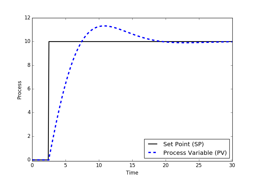
Plot the error, integral of error, and derivative of the PV for the following response. Show the value of the PID controller output and the contributions of each term to the overall output.