Concentration PID Control
 |  |  |  |  |
|---|
The objective of this case study is to use an existing dynamic model of a blending tank and develop a controller to maintain outlet concentration. A mixing tank has a liquid inlet stream and outlet stream. The tank is well mixed so the concentration is assumed to be the same throughout the reactor. The temperature is not important for this application.
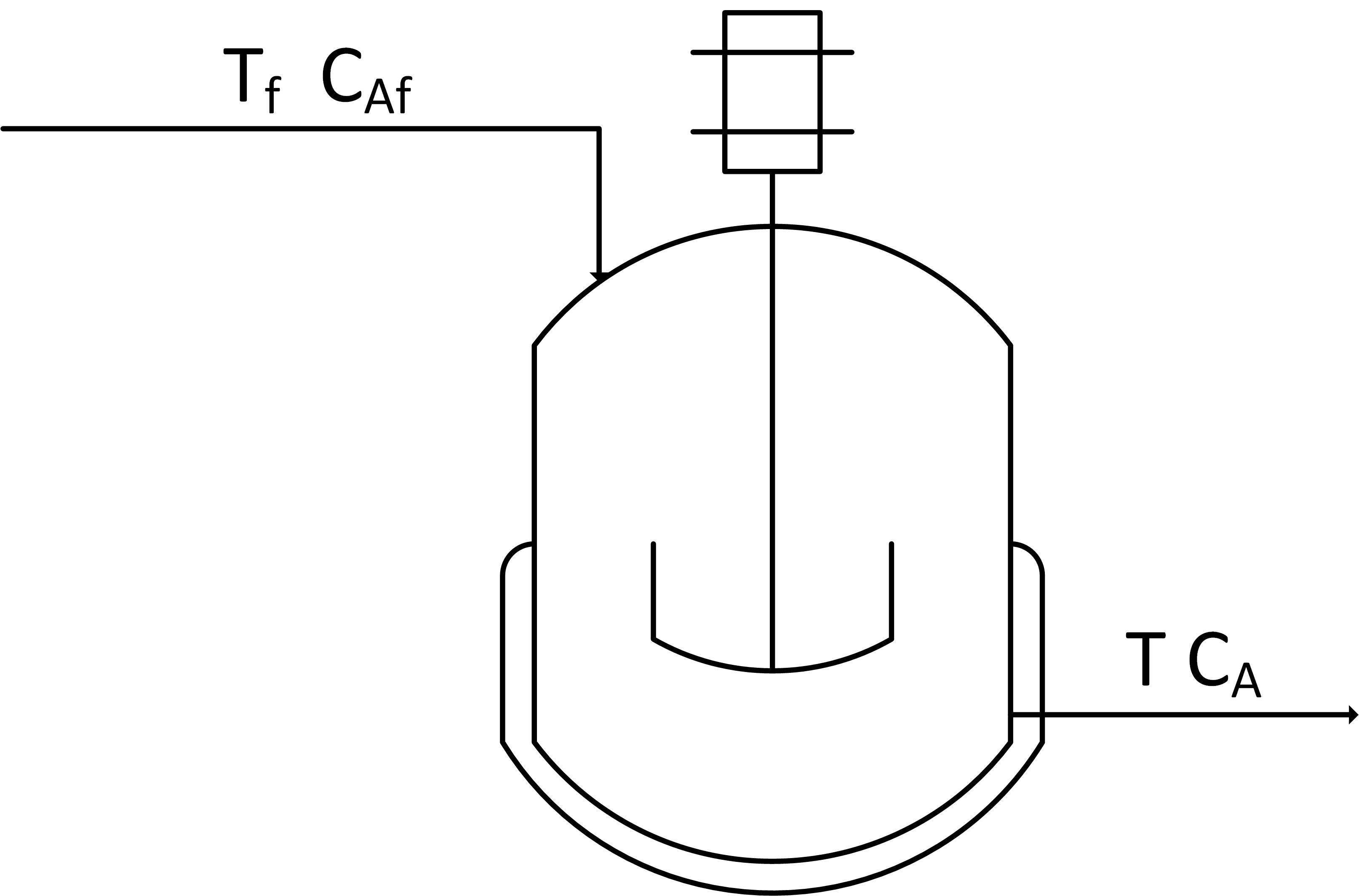
A prior exercise involves starting with species and energy balance equations and deriving the dynamic concentration and temperature response. The derivation of the concentration response is provided below with a constant tank volume V of 100 m3 and an inlet flow rate `\dot V` of 100 m3/hr. A species balance is simulated with the accumulation, inlet, and outlet terms of the number of moles n of species A. The accumulation of A, d(nA)/dt, in a control volume is calculated by inlet, outlet, reaction generation, and reaction consumption rates.
$$\frac{dn_A}{dt} = \sum \dot n_{A_{in}} - \sum \dot n_{A_{out}} + \sum \dot n_{A_{gen}} - \sum \dot n_{A_{cons}}$$
The molar amount, nA is often measured as a concentration, cA. In this application there are no reaction terms so the species balance can be simplified.
$$\frac{dc_A V}{dt} = c_{A_{in}} \dot V_{in} - c_{A_{out}} \dot V_{out}$$
Step Response Code
import matplotlib.pyplot as plt
from scipy.integrate import odeint
# define mixing model
def mixer(x,t,Tf,Caf):
# Inputs (2):
# Tf = Feed Temperature (K)
# Caf = Feed Concentration (mol/L)
# States (2):
# Concentration of A (mol/L)
Ca = x[0]
# Parameters:
# Volumetric Flowrate (m^3/hr)
q = 100
# Volume of CSTR (m^3)
V = 100
# Calculate concentration derivative
dCadt = q/V*(Caf - Ca)
return dCadt
# Initial Condition
Ca0 = 0.0
# Feed Temperature (K)
Tf = 300
# Feed Concentration (mol/L)
Caf = 1
# Time Interval (min)
t = np.linspace(0,10,100)
# Simulate mixer
Ca = odeint(mixer,Ca0,t,args=(Tf,Caf))
# Construct results and save data file
# Column 1 = time
# Column 2 = concentration
data = np.vstack((t,Ca.T)) # vertical stack
data = data.T # transpose data
np.savetxt('data.txt',data,delimiter=',')
# Plot the results
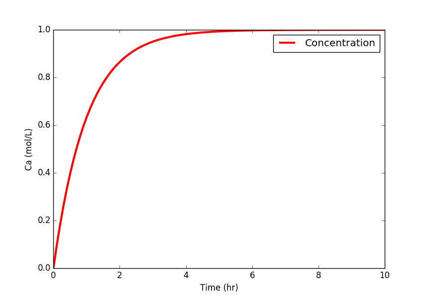
plt.plot(t,Ca,'r-',linewidth=3)
plt.ylabel('Ca (mol/L)')
plt.legend(['Concentration'],loc='best')
plt.xlabel('Time (hr)')
plt.show()
Exercise: Implement PID Control
Implement a PID controller that maintains the outlet concentration of A in the mixer by automatically adjusting the feed concentration. Assume that the concentration is continuously measured and that the controller should be designed to follow set point changes to 1.5 mol/L and then down to 1.0 mol/L. The maximum feed concentration is 2.0 mol/L and the minimum is 0.0 mol/L. Report the PID tuning parameters and show time plots of the dynamic response of the controller.
PID Solution
Generative AI Learning
Use these prompts to test your understanding after completing the exercise. Direct the AI - do not let it do the exercise for you.
App: Test the limits in the Blending Tank Control Studio. Hold the outlet concentration with PID against feed-flow and dilution upsets, and find the upset size that the 0-2 mol/L actuator constraint cannot beat. Export the CSV.
What to Turn In
Submit a short report (PDF, 1-2 pages) that curates your results into a demonstration of what you learned. You may use Generative AI to help write the report, but you must guide it to the correct visualizations, justifications, and assumptions. Answer these questions:
- Include the closed-loop response to a setpoint change and to a dilution disturbance (plots of concentration and controller output). Report your tuning.
- Show the steady-state calculation for the largest dilution upset that can still be rejected within the 0-2 mol/L constraint, and demonstrate it in simulation or the app.
- Tuning vs design: summarize in one paragraph when a control problem cannot be tuned away.
- From the quiz prompt: one question you missed and the corrected answer.