Tank Blending
 |  |  |  |
|---|
Create a dynamic model of concentration and temperature based on a physics-based derivation from species and energy balance equations. A mixing tank has a liquid inlet stream and outlet stream. The tank is well mixed so the concentration and temperature are assumed to be the same throughout the reactor.
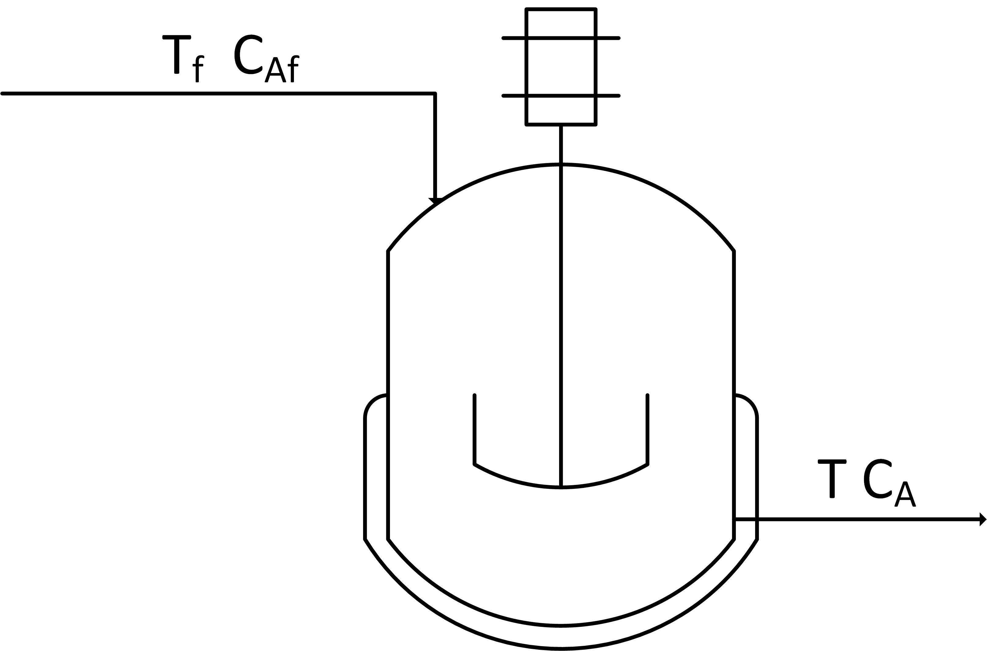
Start with the species and energy balance equations and derive the dynamic concentration and temperature response. Develop the concentration response and then add the temperature response. Assume a constant volume V of 100 m3 and an inlet flow rate `\dot V` or q of 100 m3/hr.
Solution: Species Balance
The first objective is to predict the concentration of A over a simulation time horizon. A species balance is created by relating the accumulation, inlet, and outlet terms of the number of moles n of species A. The accumulation of A, d(nA)/dt, in a control volume is calculated by inlet, outlet, reaction generation, and reaction consumption rates.
$$\frac{dn_A}{dt} = \sum \dot n_{A_{in}} - \sum \dot n_{A_{out}} + \sum \dot n_{A_{gen}} - \sum \dot n_{A_{cons}}$$
The molar amount, nA is often measured as a concentration, cA. In this application there are no reaction terms so the species balance can be simplified.
$$\frac{dc_A V}{dt} = c_{A_{in}} \dot V_{in} - c_{A_{out}} \dot V_{out}$$
import matplotlib.pyplot as plt
from scipy.integrate import odeint
# define mixing model
def mixer(x,t,Tf,Caf):
# Inputs (2):
# Tf = Feed Temperature (K)
# Caf = Feed Concentration (mol/m^3)
# States (2):
# Concentration of A (mol/m^3)
Ca = x[0]
# Parameters:
# Volumetric Flowrate (m^3/hr)
q = 100
# Volume of CSTR (m^3)
V = 100
# Calculate concentration derivative
dCadt = q/V*(Caf - Ca)
return dCadt
# Initial Condition
Ca0 = 0.0
# Feed Temperature (K)
Tf = 300
# Feed Concentration (mol/m^3)
Caf = 1
# Time Interval (min)
t = np.linspace(0,10,100)
# Simulate mixer
Ca = odeint(mixer,Ca0,t,args=(Tf,Caf))
# Construct results and save data file
# Column 1 = time
# Column 2 = concentration
data = np.vstack((t,Ca.T)) # vertical stack
data = data.T # transpose data
np.savetxt('data.txt',data,delimiter=',')
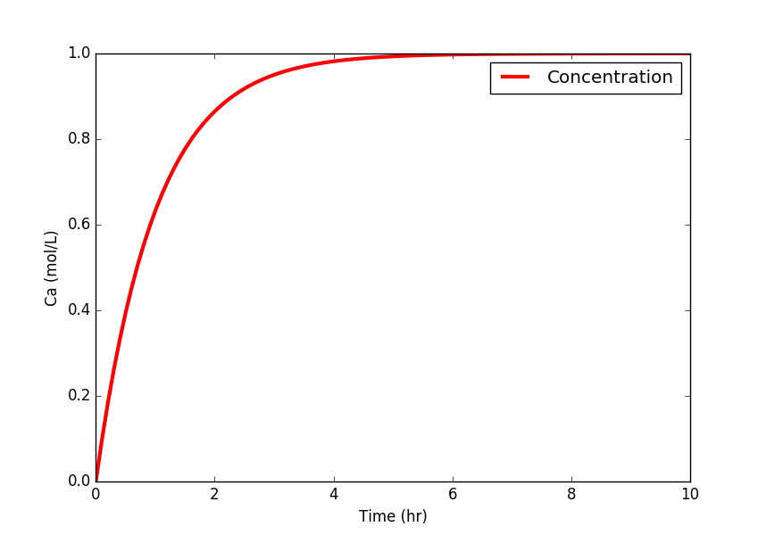
# Plot the results
plt.plot(t,Ca,'r-',linewidth=3)
plt.ylabel('Ca (mol/L)')
plt.legend(['Concentration'],loc='best')
plt.xlabel('Time (hr)')
plt.show()
Exercise: Add Energy Balance
An energy balance for this application starts with the balance equation for enthalpy, h. Enthalpy is related to temperature as m cp (T-Tref) where cp is the heat capacity. With a constant reference temperature (Tref), this reduces to the following.
$$m\,c_p\frac{dT}{dt} = \sum \dot m_{in} c_p \left( T_{in} - T_{ref} \right) - \sum \dot m_{out} c_p \left( T_{out} - T_{ref} \right) + Q + W_s$$
There is no heat input `Q`, shaft work `W_s`, or reaction. Reduce this energy balance by eliminating any terms and simplifying the expression. Implement the additional energy balance equation and simulate a feed temperature change from 350 K to 300 K. The tank fluid is initially at 350 K. The liquid heat capacity is constant and does not depend on the concentration of A.
Energy Balance Solution
TCLab Exercise
See TCLab Radiative Heat Transfer