Model Predictive Control
 |  |  |  |
|---|
Optimal control is a method to use model predictions to plan an optimized future trajectory for time-varying systems. It is often referred to as Model Predictive Control (MPC) or Dynamic Optimization. The following is an introductory video from the Dynamic Optimization Course
A method to solve dynamic control problems is by numerically integrating the dynamic model at discrete time intervals, much like measuring a physical system at particular time points. The numerical solution is compared to a desired trajectory and the difference is minimized by adjustable parameters in the model that may change at every time step. The first control action is taken and then the entire process is repeated at the next time instance. The process is repeated because objective targets may change or updated measurements may have adjusted parameter or state estimates.
Model predictive control has a number of manipulated variable (MV) and controlled variable (CV) tuning constants. The tuning constants are terms in the optimization objective function that can be adjusted to achieve a desired application performance.

As the tuning parameters are adjusted, the MPC profile is updated to reveal the effect of the change. Additional information on MPC tuning parameters is available at MPC Controller Tuning as part of the Dynamic Optimization course. There is also documentation available at Overview of APMonitor and Gekko Options. These are useful for configuring a model predictive control solution such as the vehicle model predictive control exercise.
Sequential (Shooting) MPC
Below is example MPC code in Python with Scipy.minimize.optimize instead of APMonitor and Gekko. The shooting method used in this example is generally much slower than a simultaneous method and can only be used for stable systems.
import matplotlib.pyplot as plt
import time
from scipy.integrate import odeint
from scipy.optimize import minimize
# Make an MP4 animation?
make_mp4 = False
if make_mp4:
import imageio # required to make animation
import os
try:
os.mkdir('./figures')
except:
pass
# Define process model
def process_model(y,t,u,K,tau):
# arguments
# y = outputs
# t = time
# u = input value
# K = process gain
# tau = process time constant
# calculate derivative
dydt = (-y + K * u)/(tau)
return dydt
# Define Objective function
def objective(u_hat):
# Prediction
for k in range(1,2*P+1):
if k==1:
y_hat0 = yp[i-P]
if k<=P:
if i-P+k<0:
u_hat[k] = 0
else:
u_hat[k] = u[i-P+k]
elif k>P+M:
u_hat[k] = u_hat[P+M]
ts_hat = [delta_t_hat*(k-1),delta_t_hat*(k)]
y_hat = odeint(process_model,y_hat0,ts_hat,args=(u_hat[k],K,tau))
y_hat0 = y_hat[-1]
yp_hat[k] = y_hat[0]
# Squared Error calculation
sp_hat[k] = sp[i]
delta_u_hat = np.zeros(2*P+1)
if k>P:
delta_u_hat[k] = u_hat[k]-u_hat[k-1]
se[k] = (sp_hat[k]-yp_hat[k])**2 + 20 * (delta_u_hat[k])**2
# Sum of Squared Error calculation
obj = np.sum(se[P+1:])
return obj
# FOPDT Parameters
K=3.0 # gain
tau=5.0 # time constant
ns = 100 # Simulation Length
t = np.linspace(0,ns,ns+1)
delta_t = t[1]-t[0]
# Define horizons
P = 30 # Prediction Horizon
M = 10 # Control Horizon
# Input Sequence
u = np.zeros(ns+1)
# Setpoint Sequence
sp = np.zeros(ns+1+2*P)
sp[10:40] = 5
sp[40:80] = 10
sp[80:] = 3
# Controller setting
maxmove = 1
## Process simulation
yp = np.zeros(ns+1)
# Create plot
plt.figure(figsize=(10,6))
plt.ion()
plt.show()
for i in range(1,ns+1):
if i==1:
y0 = 0
ts = [delta_t*(i-1),delta_t*i]
y = odeint(process_model,y0,ts,args=(u[i],K,tau))
y0 = y[-1]
yp[i] = y[0]
# Declare the variables in fuctions
t_hat = np.linspace(i-P,i+P,2*P+1)
delta_t_hat = t_hat[1]-t_hat[0]
se = np.zeros(2*P+1)
yp_hat = np.zeros(2*P+1)
u_hat0 = np.zeros(2*P+1)
sp_hat = np.zeros(2*P+1)
obj = 0.0
# initial guesses
for k in range(1,2*P+1):
if k<=P:
if i-P+k<0:
u_hat0[k] = 0
else:
u_hat0[k] = u[i-P+k]
elif k>P:
u_hat0[k] = u[i]
# show initial objective
print('Initial SSE Objective: ' + str(objective(u_hat0)))
# MPC calculation
start = time.time()
solution = minimize(objective,u_hat0,method='SLSQP')
u_hat = solution.x
end = time.time()
elapsed = end - start
print('Final SSE Objective: ' + str(objective(u_hat)))
print('Elapsed time: ' + str(elapsed) )
delta = np.diff(u_hat)
if i<ns:
if np.abs(delta[P]) >= maxmove:
if delta[P] > 0:
u[i+1] = u[i]+maxmove
else:
u[i+1] = u[i]-maxmove
else:
u[i+1] = u[i]+delta[P]
# plotting for forced prediction
plt.clf()
plt.subplot(2,1,1)
plt.plot(t[0:i+1],sp[0:i+1],'r-',linewidth=2,label='Setpoint')
plt.plot(t_hat[P:],sp_hat[P:],'r--',linewidth=2)
plt.plot(t[0:i+1],yp[0:i+1],'k-',linewidth=2,label='Measured CV')
plt.plot(t_hat[P:],yp_hat[P:],'k--',linewidth=2,label='Predicted CV')
plt.axvline(x=i,color='gray',alpha=0.5)
plt.axis([0, ns+P, 0, 12])
plt.ylabel('y(t)')
plt.legend()
plt.subplot(2,1,2)
plt.step(t[0:i+1],u[0:i+1],'b-',linewidth=2,label='Measured MV')
plt.plot(t_hat[P:],u_hat[P:],'b.-',linewidth=2,label='Predicted MV')
plt.axvline(x=i,color='gray',alpha=0.5)
plt.ylabel('u(t)')
plt.xlabel('time')
plt.axis([0, ns+P, 0, 6])
plt.legend()
plt.draw()
plt.pause(0.1)
if make_mp4:
filename='./figures/plot_'+str(i+10000)+'.png'
plt.savefig(filename)
# generate mp4 from png figures in batches of 350
if make_mp4:
images = []
iset = 0
for i in range(1,ns):
filename='./figures/plot_'+str(i+10000)+'.png'
images.append(imageio.imread(filename))
if ((i+1)%350)==0:
imageio.mimsave('results_'+str(iset)+'.mp4', images)
iset += 1
images = []
if images!=[]:
imageio.mimsave('results_'+str(iset)+'.mp4', images)
Industrial MPC
There are many applications of model predictive control and optimization with Gekko. One example is nonlinear Model Predictive Control (MPC) for 💦 water recovery in tailings reprocessing in South Africa.
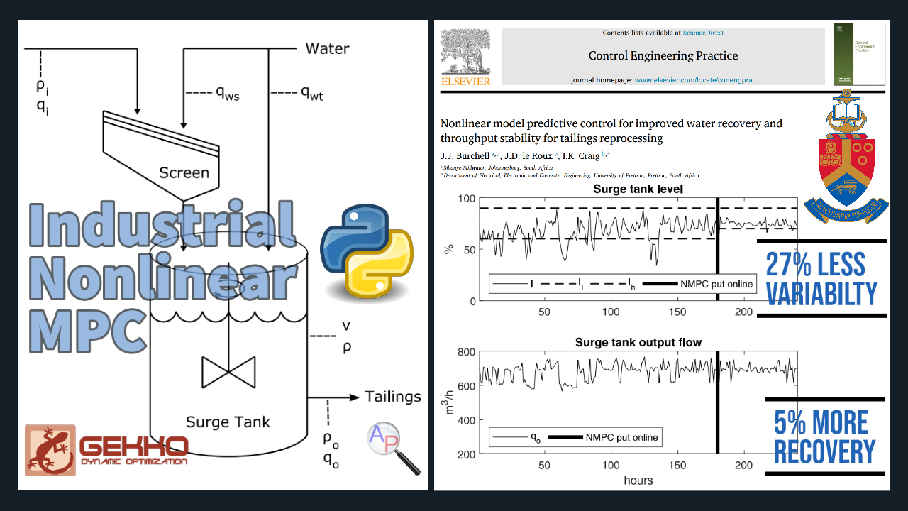
There is a 27% decrease in variability and 5% increase in water recovery. Read the full report in the recently published article by J.J. Burchell, J.D. le Roux, and Ian K Craig at the University of Pretoria in South Africa.
Additional Information
- Burchell, J.J., le Roux, J.D., Craig, I.K., Nonlinear model predictive control for improved water recovery and throughput stability for tailings reprocessing, Control Engineering Practice, Volume 131, 2023, 105385, ISSN 0967-0661, DOI: 10.1016/j.conengprac.2022.105385. Article
- Vehicle MPC (Simple MPC Application)
- Hot Air Balloon MPC
- Gekko Documentation
- Gekko Example Applications