Dynamic controller tuning is the process of adjusting certain objective function terms to give more desirable solutions. As an example, a dynamic control application may either exhibit too aggressive manipulated variable movement or be too sluggish during set-point changes. Tuning is the iterative process of finding acceptable values that work over a wide range of operating conditions.

MPC Tuning IPython Widget

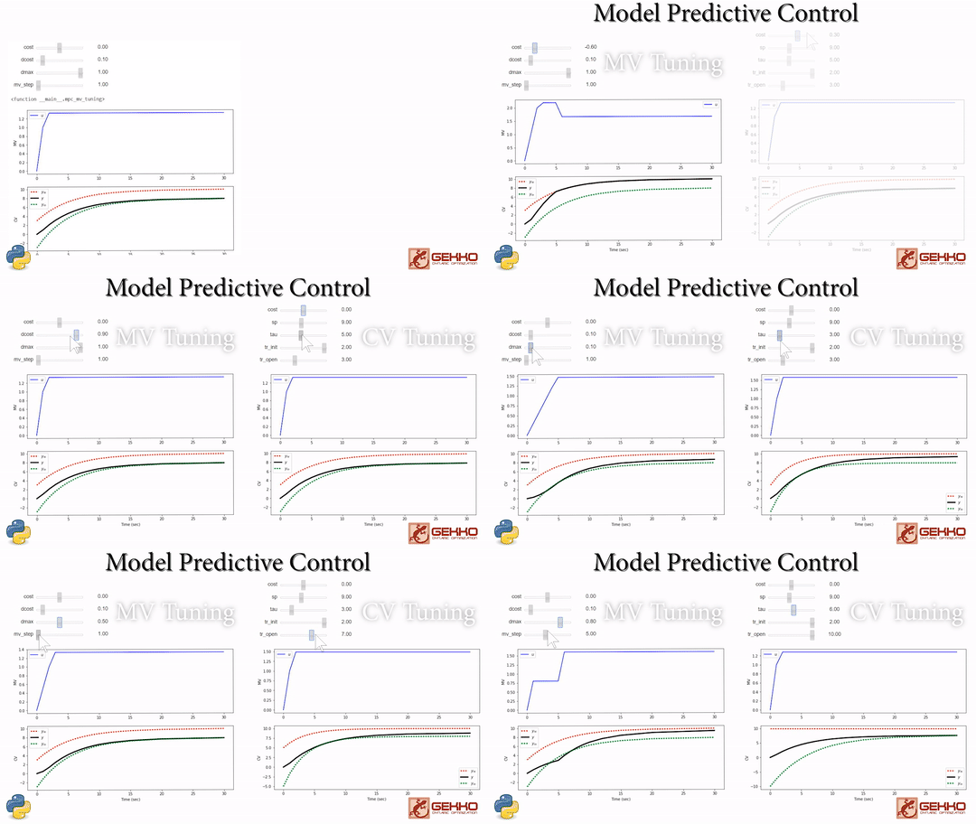
Common Tuning Parameters for MPC

Tuning typically involves adjustment of objective function terms or constraints that limit the rate of change (DMAX), penalize the rate of change (DCOST), or set absolute bounds (LOWER and UPPER). Measurement availability is indicated by the parameter (FSTATUS). The optimizer can also include (1=on) or exclude (0=off) a certain manipulated variable (MV) or controlled variable with STATUS. Below are common application, MV, and CV tuning constants that are adjusted to achieve desired model predictive control performance.

• Application tuning
  • IMODE = 6 or 9 for model predictive control
  • CV_TYPE = CV type with 1=l_1-norm, 2=squared error
  • DIAGLEVEL = diagnostic level (0-10) for solution information
  • MAX_ITER = maximum iterations
  • MAX_TIME = maximum time before stopping
  • MV_TYPE = Set default MV type with 0=zero-order hold, 1=linear interpolation
  • SOLVER
    • 0=Try all available solvers
    • 1=APOPT (MINLP, Active Set SQP)
    • 2=BPOPT (NLP, Interior Point, SQP)
    • 3=IPOPT (NLP, Interior Point, SQP)
• Manipulated Variable (MV) tuning
  • COST = (+) minimize MV, (-) maximize MV
  • DCOST = penalty for MV movement
  • DMAX = maximum that MV can move each cycle
  • FSTATUS = feedback status with 1=measured, 0=off
  • LOWER = lower MV bound
  • MV_TYPE = MV type with 0=zero-order hold, 1=linear interpolation
  • STATUS = turn on (1) or off (0) MV
  • UPPER = upper MV bound
• Controlled Variable (CV) tuning
  • COST = (+) minimize CV, (-) maximize CV
  • FSTATUS = feedback status with 1=measured, 0=off
  • SP = set point with CV_TYPE = 2
  • SPLO = lower set point with CV_TYPE = 1
  • SPHI = upper set point with CV_TYPE = 1
  • STATUS = turn on (1) or off (0) CV
  • TAU = reference trajectory time-constant
  • TR_INIT = trajectory type, 0=dead-band, 1,2=trajectory
  • TR_OPEN = opening at initial point of trajectory compared to end

There are several ways to change the tuning values. Tuning values can either be specified before an application is initialized or while an application is running. To change a tuning value before the application is loaded, use the apm_option() function such as the following example to change the lower bound in MATLAB or Python for the MV named u.

 apm_option(server,app,'u.LOWER',0)

The upper and lower deadband targets for a CV named y are set to values around a desired set point of 10.0. In this case, an acceptable range for this CV is between 9.5 and 10.5.

 sp = 10.0
 apm_option(server,app,'y.SPHI',sp+0.5)
 apm_option(server,app,'y.SPHI',sp-0.5)

Application constants are modified by indicating that the constant belongs to the group nlc. IMODE is adjusted to either solve the MPC problem with a simultaneous (6) or sequential (9) method. In the case below, the application IMODE is changed to simultaneous mode.

 apm_option(server,app,'nlc.IMODE',6)

Exercise 1

Objective: Design a model predictive controller with one manipulated variable and two controlled variables with competing objectives that cannot be simultaneously satisfied. Tune the controller to achieve best performance. Estimated time: 2 hours.

Use the following system of linear differential equations for this exercise by placing the model definition in the file myModel.apm (APMonitor) or in a Python script (Gekko).

APMonitor Model

 Parameters
  u
 Variables
  x
  y
 Equations
  5 * $x = -x + 1.5 * u
  15 * $y = -y + 3.0 * u

Gekko Model

In this case, the parameter u is the manipulated variable and x and y are the controlled variables. It is desired to maximize x and maintain values between 9 and 10. It is desired to maintain values of y between 2 and 7. For the first 10 minutes, the priority is to maintain the range for y and following this time period, it is desired to track the range for x. Tune the controller to meet these objectives while minimizing MV movement.

Solution

MPC Tuning Solution (APM MATLAB and APM Python

Exercise 2 — Surge Tank Level and Density Control

Objective: Design and tune an MPC that regulates (1) tank level within safe bounds and (2) product density to a target range despite feed-density disturbances. Use dilution-water flow as the single MV. Estimated time: 2–3 hours.

Process Description A cylindrical surge tank blends a dense slurry with dilution water. The outflow goes to a downstream unit that requires stable level and density.

• Geometry
  • Tank height: H = 3.0 m
  • Tank diameter: D = 2.0 m
  • Cross-sectional area: A = πD²/4
• Flows (m³/min)
  • Q_W: dilution-water inflow (MV)
  • Q_S: slurry inflow (disturbance)
  • Q_P: product outflow
• States
  • Mass M (t) and volume V (m³)
  • Level (%): L = 100·V/(A·H)
  • Product density (kg/L): ρ_P = M/V
  • Water density ρ_W = 1.0 kg/L, slurry density ρ_S ≈ 2.0 kg/L + disturbances

Nonlinear Plant Model (mass/volume balances)

 dM/dt = Q_W·ρ_W + Q_S·ρ_S − Q_P·ρ_P
 dV/dt = Q_W + Q_S − Q_P
 L = 100·V/(A·H),  ρ_P = M/V

When L ≤ 0% or L ≥ 100%, hold dV/dt = 0 to avoid unphysical overflow/emptying during simulation.

Internal MPC Model A simplified internal model suitable for control design (you may keep the nonlinear balances as the “plant” simulator):

• Level integrator (relative to Q_W* where * is steady state): (A·H)·(dL/dt) = 100·(Q_W − Q_W*)
• First-order density response to dilution water: τ_model·(dρ_P/dt) = −(ρ_P − ρ_P*) + K_p·(Q_W − Q_W*) with K_p ≈ −0.24 (kg·L⁻¹)/(m³·min⁻¹), τ_model ≈ 0.8 min

Controller Design

• MV: dilution-water flow Q_W
  • Bounds: 0.0 ≤ Q_W ≤ 1.6 m³/min (adjust as needed)
  • Movement limits: DMAX ≈ 0.1–0.3 m³/min per move
  • Movement penalty: DCOST ≈ 0.02–0.10
• CVs:
  • Level L (%): Safety-critical. Keep within 20–80% at all times.
    • Use deadband tracking (CV_TYPE=1) with SPLO=20, SPHI=80.
    • Heavier penalties on violating bounds (e.g., WSPLO=WSPHI ≫ density weights).
  • Product density ρ_P (kg/L): Quality target 1.60 ± 0.05.
    • Deadband tracking with SPLO=1.55, SPHI=1.65 (optionally a small buffer inside these hard limits).
    • Moderate weight relative to level.
• Priority / Importance
  • Level (safety) > Density (quality) > MV movement.
  • Example weights: L.WSPLO=L.WSPHI=10 (or higher if needed); ρ_P.WSPLO=ρ_P.WSPHI=1.
• Timing
  • Controller interval: 1.0 min; prediction horizon ≈ 10–15 min; NODES≈2–3.

Disturbance Scenarios

1. Random-walk changes in ρ_S with σ ≈ 0.018 kg/L per step (every 0.2 min).
2. Optional steps: at t = 30 min, ρ_S → 2.10; at t = 60 min, ρ_S → 1.90.

Tasks

1. Implement the internal MPC model (level integrator + first-order density).
2. Tune DMAX, DCOST, and CV weights to:
   1. keep L within 20–80% at all times (no overflow/empty),
   2. keep ρ_P within 1.60 ± 0.05 after disturbances (settle < ~3–5 min),
   3. avoid excessive Q_W movement.

```

Full Solution

Thanks to Vincent Roos for the Level and Density control exercise and Gekko solution.

Discussion Questions

1. A hard upper bound on a controlled state and a soft constraint with a large violation penalty can produce the same closed-loop trajectory in nominal operation. Under what disturbance do they behave completely differently, and which failure mode do you prefer in a real plant?
2. The squared-error objective (CV_TYPE=2) with a reference trajectory and the l1 deadband objective (CV_TYPE=1) both "track a setpoint." Which one keeps moving the MV when the CV sits inside a noise band, and what does that cost in actuator life?
3. DMAX and DCOST both slow the manipulated variable. One is a constraint, one is a price. Which one can make the problem infeasible, which one degrades gracefully, and when would you use each?
4. Increasing TAU on the reference trajectory and increasing DCOST on the MV both make the response gentler. How would you tell from closed-loop data which one a previous engineer used?

Generative AI Learning

Use these prompts with the tuning exercises (competing CVs, and the surge tank level/density problem). Direct the AI - the tuning tradeoffs are engineering judgment, which is the deliverable.

What to Turn In

Submit a short report (PDF, 1-2 pages) that curates your results into a demonstration of what you learned. You may use Generative AI to help write the report, but you must guide it to the correct visualizations, justifications, and assumptions. Answer these questions:

1. Exercise 1: show the two-CV solution with the time-based priority switch, and explain which tuning values enforce the priority and how the MV movement was kept minimal.
2. Exercise 2 (surge tank): include level and density plots against the feed disturbances, your final tuning table, and one sentence per parameter on why that value.
3. Demonstrate one hard-vs-soft constraint comparison on the tank level: same disturbance, both formulations. What differs in the trajectories and in solver behavior?
4. From the reviewer prompt: the disturbance scenario that broke (or nearly broke) your tuning, and what you changed in response.