Rocket Launch: Classic Optimal Control
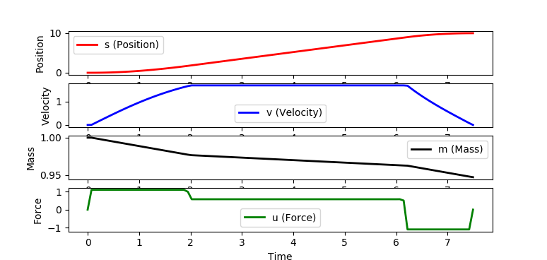
A rocket burn trajectory is desired to minimize a travel time between a starting point and a final point, 10 units of distance away. The thrust can be between an upper limit of 1.1 and a lower limit of -1.1. The initial and final velocity must be zero and the maximum velocity can never exceed 1.7. It is also desirable to minimize the use of fuel to perform the maneuver. There is a drag resistance the is proportional to the square of the velocity and mass is lost as the fuel is burned during thrust operations.
Problem Statement
 minimize tf

 subject to
   ds/dt = v
   dv/dt = (u-0.2*v^2)/m
   dm/dt = -0.01 * u^2

 path constraints
   0.0 <= v(t) <= 1.7
   -1.1 <= u(t) <= 1.1

 initial boundary conditions
   s(0) = 0
   v(0) = 0
   m(0) = 1

 final boundary conditions
   s(tf) = 10.0
   v(tf) = 0.0
APM MATLAB and APM Python Solution

Python GEKKO Solution
The GEKKO package is available through the package manager pip in Python.
python -m pip install gekko
GEKKO Python is designed for large-scale optimization and accesses solvers of constrained, unconstrained, continuous, and discrete problems.
import numpy as np
import matplotlib.pyplot as plt
from gekko import GEKKO
# create GEKKO model
m = GEKKO()
# scale 0-1 time with tf
m.time = np.linspace(0,1,101)
# options
m.options.NODES = 6
m.options.SOLVER = 3
m.options.IMODE = 6
m.options.MAX_ITER = 500
m.options.MV_TYPE = 0
m.options.DIAGLEVEL = 0
# final time
tf = m.FV(value=1.0,lb=0.1,ub=100)
tf.STATUS = 1
# force
u = m.MV(value=0,lb=-1.1,ub=1.1)
u.STATUS = 1
u.DCOST = 1e-5
# variables
s = m.Var(value=0)
v = m.Var(value=0,lb=0,ub=1.7)
mass = m.Var(value=1,lb=0.2)
# differential equations scaled by tf
m.Equation(s.dt()==tf*v)
m.Equation(mass*v.dt()==tf*(u-0.2*v**2))
m.Equation(mass.dt()==tf*(-0.01*u**2))
# specify endpoint conditions
m.fix(s, pos=len(m.time)-1,val=10.0)
m.fix(v, pos=len(m.time)-1,val=0.0)
# minimize final time
m.Obj(tf)
# Optimize launch
m.solve()
print('Optimal Solution (final time): ' + str(tf.value[0]))
# scaled time
ts = m.time * tf.value[0]
# plot results
plt.figure(1)
plt.subplot(4,1,1)
plt.plot(ts,s.value,'r-',lw=2)
plt.ylabel('Position')
plt.legend(['s (Position)'])
plt.subplot(4,1,2)
plt.plot(ts,v.value,'b-',lw=2)
plt.ylabel('Velocity')
plt.legend(['v (Velocity)'])
plt.subplot(4,1,3)
plt.plot(ts,mass.value,'k-',lw=2)
plt.ylabel('Mass')
plt.legend(['m (Mass)'])
plt.subplot(4,1,4)
plt.plot(ts,u.value,'g-',lw=2)
plt.ylabel('Force')
plt.legend(['u (Force)'])
plt.xlabel('Time')
plt.show()