TCLab B - MIMO Digital Twin
The TCLab is a hands-on application of machine learning and advanced temperature control with two heaters and two temperature sensors. The labs reinforce principles of model development, estimation, and advanced control methods. This is the second exercise to simulate an energy balance and compare the predictions to deep learning with a multi-layered neural network. The additional feature over the first lab is that the model is extended to two heaters and two temperature sensors.
Lab Problem Statement
Data and Solutions
- MIMO Energy Balance Solution with MATLAB and Python
- Steady state data, 2 heaters
- Dynamic data, 2 heaters
import pandas as pd
import tclab
import time
import matplotlib.pyplot as plt
# generate step test data on Arduino
filename = 'tclab_dyn_data2.csv'
# heater steps
Q1d = np.zeros(601)
Q1d[10:200] = 80
Q1d[200:280] = 20
Q1d[280:400] = 70
Q1d[400:] = 50
Q2d = np.zeros(601)
Q2d[120:320] = 100
Q2d[320:520] = 10
Q2d[520:] = 80
# Connect to Arduino
a = tclab.TCLab()
fid = open(filename,'w')
fid.write('Time,H1,H2,T1,T2\n')
fid.close()
# run step test (10 min)
for i in range(601):
# set heater values
a.Q1(Q1d[i])
a.Q2(Q2d[i])
print('Time: ' + str(i) + \
' H1: ' + str(Q1d[i]) + \
' H2: ' + str(Q2d[i]) + \
' T1: ' + str(a.T1) + \
' T2: ' + str(a.T2))
# wait 1 second
time.sleep(1)
fid = open(filename,'a')
fid.write(str(i)+','+str(Q1d[i])+','+str(Q2d[i])+',' \
+str(a.T1)+','+str(a.T2)+'\n')
# close connection to Arduino
a.close()
# read data file
data = pd.read_csv(filename)
# plot measurements
plt.figure()
plt.subplot(2,1,1)
plt.plot(data['Time'],data['H1'],'r-',label='Heater 1')
plt.plot(data['Time'],data['H2'],'b--',label='Heater 2')
plt.ylabel('Heater (%)')
plt.legend(loc='best')
plt.subplot(2,1,2)
plt.plot(data['Time'],data['T1'],'r.',label='Temperature 1')
plt.plot(data['Time'],data['T2'],'b.',label='Temperature 2')
plt.ylabel('Temperature (degC)')
plt.legend(loc='best')
plt.xlabel('Time (sec)')
plt.savefig('tclab_dyn_meas2.png')
plt.show()
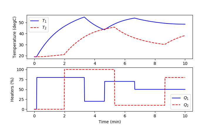
import matplotlib.pyplot as plt
from gekko import GEKKO
#initialize GEKKO model
m = GEKKO()
#model discretized time
n = 60*10+1 # Number of second time points (10min)
m.time = np.linspace(0,n-1,n) # Time vector
# Parameters
# Percent Heater (0-100%)
Q1d = np.zeros(n)
Q1d[10:200] = 80
Q1d[200:280] = 20
Q1d[280:400] = 70
Q1d[400:] = 50
Q1 = m.Param()
Q1.value = Q1d
Q2d = np.zeros(n)
Q2d[120:320] = 100
Q2d[320:520] = 10
Q2d[520:] = 80
Q2 = m.Param()
Q2.value = Q2d# Heaters as time-varying inputs
Q1 = m.Param(value=Q1d) # Percent Heater (0-100%)
Q2 = m.Param(value=Q2d) # Percent Heater (0-100%)
T0 = m.Param(value=19.0+273.15) # Initial temperature
Ta = m.Param(value=19.0+273.15) # K
U = m.Param(value=10.0) # W/m^2-K
mass = m.Param(value=4.0/1000.0) # kg
Cp = m.Param(value=0.5*1000.0) # J/kg-K
A = m.Param(value=10.0/100.0**2) # Area not between heaters in m^2
As = m.Param(value=2.0/100.0**2) # Area between heaters in m^2
alpha1 = m.Param(value=0.01) # W / % heater
alpha2 = m.Param(value=0.005) # W / % heater
eps = m.Param(value=0.9) # Emissivity
sigma = m.Const(5.67e-8) # Stefan-Boltzman
# Temperature states as GEKKO variables
T1 = m.Var(value=T0)
T2 = m.Var(value=T0)
# Between two heaters
Q_C12 = m.Intermediate(U*As*(T2-T1)) # Convective
Q_R12 = m.Intermediate(eps*sigma*As*(T2**4-T1**4)) # Radiative
m.Equation(T1.dt() == (1.0/(mass*Cp))*(U*A*(Ta-T1) \
+ eps * sigma * A * (Ta**4 - T1**4) \
+ Q_C12 + Q_R12 \
+ alpha1*Q1))
m.Equation(T2.dt() == (1.0/(mass*Cp))*(U*A*(Ta-T2) \
+ eps * sigma * A * (Ta**4 - T2**4) \
- Q_C12 - Q_R12 \
+ alpha2*Q2))
#simulation mode
m.options.IMODE = 4
#simulation model
m.solve()
#plot results
plt.figure(1)
plt.subplot(2,1,1)
plt.plot(m.time/60.0,np.array(T1.value)-273.15,'b-')
plt.plot(m.time/60.0,np.array(T2.value)-273.15,'r--')
plt.legend([r'$T_1$',r'$T_2$'],loc='best')
plt.ylabel('Temperature (degC)')
plt.subplot(2,1,2)
plt.plot(m.time/60.0,np.array(Q1.value),'b-')
plt.plot(m.time/60.0,np.array(Q2.value),'r--')
plt.legend([r'$Q_1$',r'$Q_2$'],loc='best')
plt.ylabel('Heaters (%)')
plt.xlabel('Time (min)')
plt.show()
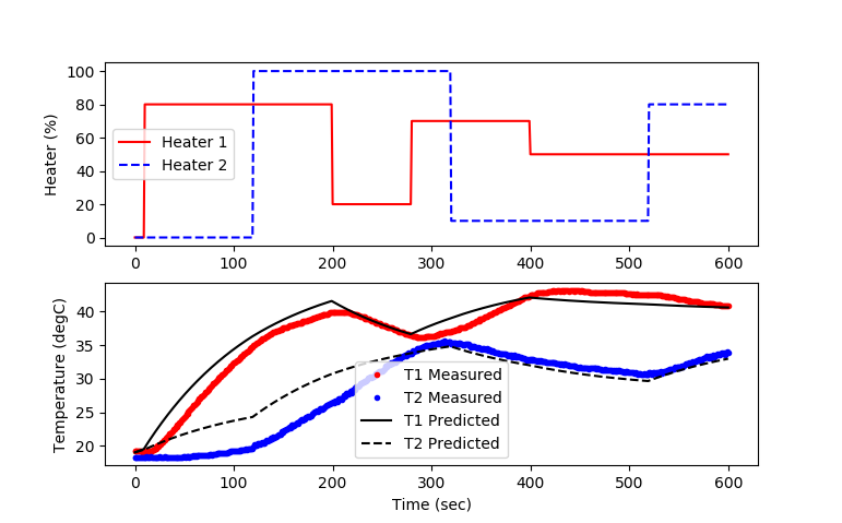
import pandas as pd
import matplotlib.pyplot as plt
from sklearn.preprocessing import MinMaxScaler
from gekko import GEKKO
import time
# -------------------------------------
# import or generate data
# -------------------------------------
filename = 'tclab_ss_data2.csv'
try:
try:
data = pd.read_csv(filename)
except:
url = 'https://apmonitor.com/do/uploads/Main/tclab_ss_data2.txt'
data = pd.read_csv(url)
except:
# generate training data if data file not available
import tclab
# Connect to Arduino
a = tclab.TCLab()
fid = open(filename,'w')
fid.write('Heater 1,Heater 2,Temperature 1,Temperature 2\n')
fid.close()
# data collection takes 6 hours = 120 pts * 3 minutes each
npts = 120
for i in range(npts):
# set random heater values
Q1 = np.random.rand()*100
Q2 = np.random.rand()*100
a.Q1(Q1)
a.Q2(Q2)
print('Heater 1: ' + str(Q1) + ' %')
print('Heater 2: ' + str(Q2) + ' %')
# wait 3 minutes
time.sleep(3*60)
# record temperature and heater value
print('Temperature 1: ' + str(a.T1) + ' degC')
print('Temperature 2: ' + str(a.T2) + ' degC')
fid = open(filename,'a')
fid.write(str(Q1)+','+str(Q2)+','+str(a.T1)+','+str(a.T2)+'\n')
fid.close()
# close connection to Arduino
a.close()
# read data file
data = pd.read_csv(filename)
# -------------------------------------
# scale data
# -------------------------------------
s = MinMaxScaler(feature_range=(0,1))
sc_train = s.fit_transform(data)
# partition into inputs and outputs
xs = sc_train[:,0:2] # 2 heaters
ys = sc_train[:,2:4] # 2 temperatures
# -------------------------------------
# build neural network
# -------------------------------------
nin = 2 # inputs
n1 = 2 # hidden layer 1 (linear)
n2 = 2 # hidden layer 2 (nonlinear)
n3 = 2 # hidden layer 3 (linear)
nout = 2 # outputs
# Initialize gekko models
train = GEKKO()
dyn = GEKKO()
model = [train,dyn]
for m in model:
# use APOPT solver
m.options.SOLVER = 1
# input(s)
m.inpt = [m.Param() for i in range(nin)]
# layer 1 (linear)
m.w1 = m.Array(m.FV, (nout,nin,n1))
m.l1 = [[m.Intermediate(sum([m.w1[k,j,i]*m.inpt[j] \
for j in range(nin)])) for i in range(n1)] \
for k in range(nout)]
# layer 2 (tanh)
m.w2 = m.Array(m.FV, (nout,n1,n2))
m.l2 = [[m.Intermediate(sum([m.tanh(m.w2[k,j,i]*m.l1[k][j]) \
for j in range(n1)])) for i in range(n2)] \
for k in range(nout)]
# layer 3 (linear)
m.w3 = m.Array(m.FV, (nout,n2,n3))
m.l3 = [[m.Intermediate(sum([m.w3[k,j,i]*m.l2[k][j] \
for j in range(n2)])) for i in range(n3)] \
for k in range(nout)]
# outputs
m.outpt = [m.CV() for i in range(nout)]
m.Equations([m.outpt[k]==sum([m.l3[k][i] for i in range(n3)]) \
for k in range(nout)])
# flatten matrices
m.w1 = m.w1.flatten()
m.w2 = m.w2.flatten()
m.w3 = m.w3.flatten()
# -------------------------------------
# fit parameter weights
# -------------------------------------
m = train
for i in range(nin):
m.inpt[i].value=xs[:,i]
for i in range(nout):
m.outpt[i].value = ys[:,i]
m.outpt[i].FSTATUS = 1
for i in range(len(m.w1)):
m.w1[i].FSTATUS=1
m.w1[i].STATUS=1
m.w1[i].MEAS=1.0
for i in range(len(m.w2)):
m.w2[i].STATUS=1
m.w2[i].FSTATUS=1
m.w2[i].MEAS=0.5
for i in range(len(m.w3)):
m.w3[i].FSTATUS=1
m.w3[i].STATUS=1
m.w3[i].MEAS=1.0
m.options.IMODE = 2
m.options.EV_TYPE = 2
# solve for weights to minimize loss (objective)
m.solve(disp=True)
# -------------------------------------
# generate dynamic predictions
# -------------------------------------
m = dyn
tf = 600
m.time = np.linspace(0,tf,tf+1)
# load neural network parameters
for i in range(len(m.w1)):
m.w1[i].MEAS=train.w1[i].NEWVAL
m.w1[i].FSTATUS = 1
for i in range(len(m.w2)):
m.w2[i].MEAS=train.w2[i].NEWVAL
m.w2[i].FSTATUS = 1
for i in range(len(m.w3)):
m.w3[i].MEAS=train.w3[i].NEWVAL
m.w3[i].FSTATUS = 1
# step tests
Q1d = np.zeros(tf+1)
Q1d[10:200] = 80
Q1d[200:280] = 20
Q1d[280:400] = 70
Q1d[400:] = 50
Q1 = m.Param()
Q1.value = Q1d
Q2d = np.zeros(tf+1)
Q2d[120:320] = 100
Q2d[320:520] = 10
Q2d[520:] = 80
Q2 = m.Param()
Q2.value = Q2d
# scaled inputs
m.inpt[0].value = Q1d * s.scale_[0] + s.min_[0]
m.inpt[1].value = Q2d * s.scale_[1] + s.min_[1]
# define Temperature output
Q0 = 0 # initial heater
T0 = 19 # ambient temperature
# scaled steady state ouput
T1_ss = m.Var(value=T0)
T2_ss = m.Var(value=T0)
m.Equation(T1_ss == (m.outpt[0]-s.min_[2])/s.scale_[2])
m.Equation(T2_ss == (m.outpt[1]-s.min_[3])/s.scale_[3])
# dynamic prediction
T1 = m.Var(value=T0)
T2 = m.Var(value=T0)
# time constant
tau = m.Param(value=120) # determine in a later exercise
# additional model equation for dynamics
m.Equation(tau*T1.dt()==-(T1-T0)+(T1_ss-T0))
m.Equation(tau*T2.dt()==-(T2-T0)+(T2_ss-T0))
# solve dynamic simulation
m.options.IMODE=4
m.solve()
# generate step test data on Arduino
# -------------------------------------
# import or generate data
# -------------------------------------
filename = 'tclab_dyn_data2.csv'
try:
try:
data = pd.read_csv(filename)
except:
url = 'https://apmonitor.com/do/uploads/Main/tclab_dyn_data2.txt'
data = pd.read_csv(url)
except:
# generate training data if data file not available
import tclab
# Connect to Arduino
a = tclab.TCLab()
fid = open(filename,'w')
fid.write('Time,H1,H2,T1,T2\n')
fid.close()
# check for cool down
i = 0
while i<=10:
i += 1 # upper limit on wait time
T1m = a.T1
T2m = a.T2
print('T1: ' + str(a.T1) + ' T2: ' + str(a.T2))
print('Sleep 30 sec')
time.sleep(30)
if (a.T1<30 and a.T2<30 and a.T1>=T1m-0.2 and a.T2>=T2m-0.2):
break # continue when conditions met
else:
print('Not at ambient temperature')
# run step test (10 min)
for i in range(tf+1):
# set heater values
a.Q1(Q1d[i])
a.Q2(Q2d[i])
print('Time: ' + str(i) + \
' H1: ' + str(Q1d[i]) + \
' H2: ' + str(Q2d[i]) + \
' T1: ' + str(a.T1) + \
' T2: ' + str(a.T2))
# wait 1 second
time.sleep(1)
fid = open(filename,'a')
fid.write(str(i)+','+str(Q1d[i])+','+str(Q2d[i])+',' \
+str(a.T1)+','+str(a.T2)+'\n')
fid.close()
# close connection to Arduino
a.close()
# read data file
data = pd.read_csv(filename)
# plot prediction and measurement
plt.figure()
plt.subplot(2,1,1)
plt.plot(m.time,Q1.value,'r-',label='Heater 1')
plt.plot(m.time,Q2.value,'b--',label='Heater 2')
plt.ylabel('Heater (%)')
plt.legend(loc='best')
plt.subplot(2,1,2)
plt.plot(data['Time'],data['T1'],'r.',label='T1 Measured')
plt.plot(data['Time'],data['T2'],'b.',label='T2 Measured')
plt.plot(m.time,T1.value,'k-',label='T1 Predicted')
plt.plot(m.time,T2.value,'k--',label='T2 Predicted')
plt.ylabel('Temperature (degC)')
plt.legend(loc='best')
plt.xlabel('Time (sec)')
plt.savefig('tclab_dyn_pred.png')
plt.show()
See also:
Generative AI Learning
Use these prompts around the MIMO lab. Predict the coupling before you measure it - that is the heart of a multivariable model.
App: The two-heater extension of the TCLab Simulation Studio fits the MIMO energy balance with sliders - use it to sanity-check your coupling parameters against your CSV before trusting the optimizer.
What to Turn In
Submit a short report (PDF, 1-2 pages) that curates your results into a demonstration of what you learned. You may use Generative AI to help write the report, but you must guide it to the correct visualizations, justifications, and assumptions. Answer these questions:
- Show measured vs predicted T1 and T2 for a step test that exercises both heaters, for the physics-based model and the neural network. Label hardware vs simulated data.
- Quantify the largest mismatch in the cross-coupling (Q1 to T2 or Q2 to T1) and defend it physically. Which coupling mechanism (convective vs radiative vs board conduction) does your data implicate, and why?
- Your written coupling prediction vs the measurement: where was your physical reasoning wrong, and what number fixed it?
- The neural network fits the training data better. Give one concrete input scenario from your own data range's edge where you trust the energy balance more, and justify.