Arduino Dynamic Response: 2 Heaters
Objective: Derive a nonlinear transient model for two heaters and compare the model predictions with the Arduino temperature control lab measurements.
A next step in the modeling, beyond the single heater model, is to develop a dual heater model and add the heat transfer between them. The temperature control lab has two transistor heaters and two temperature sensors as shown in the figure below.
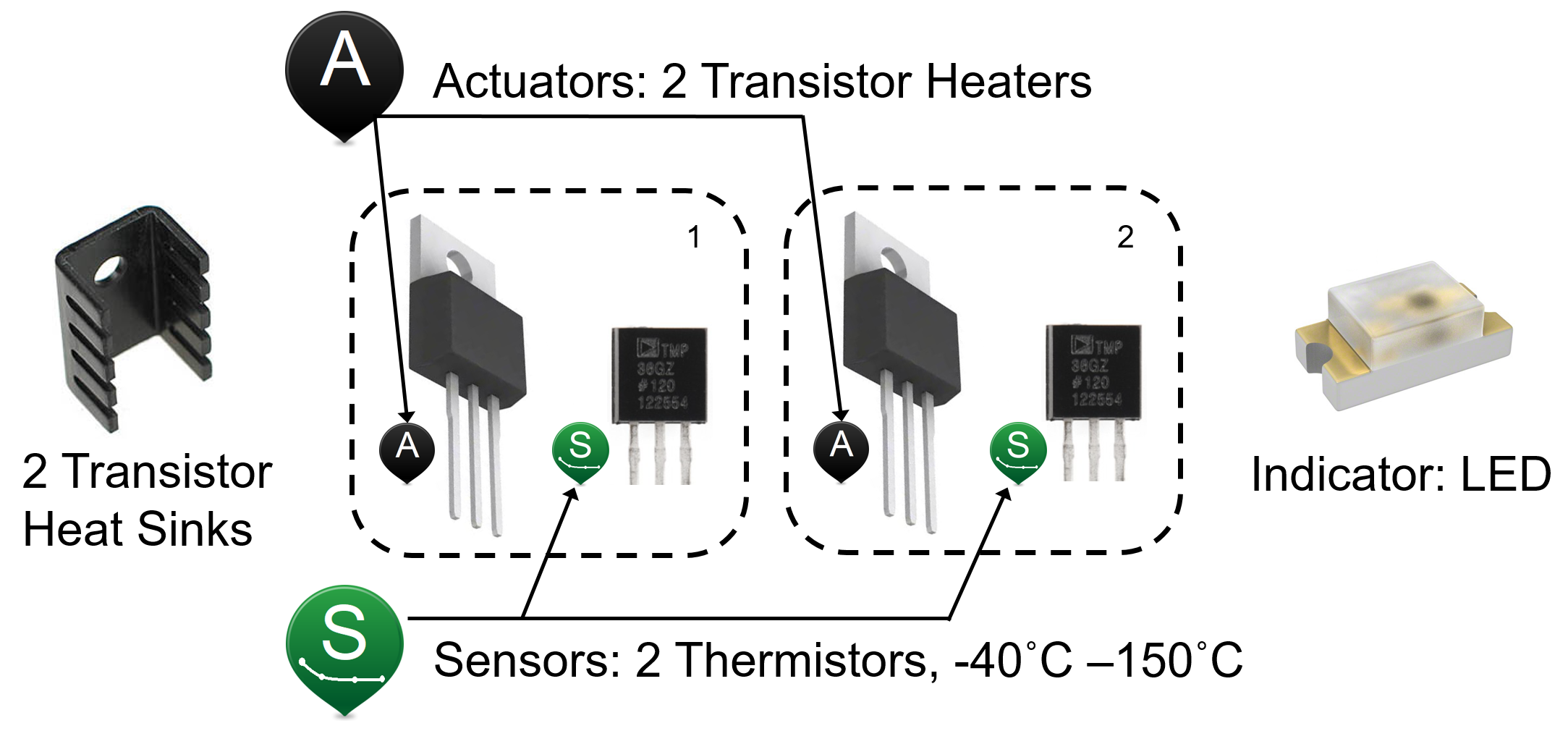
The model for the dual heater system is similar to the single heater model except that the surface is further differentiated for area that is between the two heaters (2 cm2) and the area that is not coupled between the heaters (10 cm2). Also, heater 2 dissipates a maximum of 0.75 W while heater 1 dissipates a maximum of 1.0 W.
| Quantity | Value |
| Initial temperature (T0) | 296.15 K (23oC) |
| Ambient temperature (`T_\infty`) | 296.15 K (23oC) |
| Heater output (Q1) | 0 to 1 W |
| Heater factor (`\alpha_1`) | 0.01 W/(% heater) |
| Heater output (Q2) | 0 to 0.75 W |
| Heater factor (`\alpha_2`) | 0.0075 W/(% heater) |
| Heat capacity (Cp) | 500 J/kg-K |
| Surface Area Not Between Heaters (A) | 1.0x10⁻³ m2 (10 cm2) |
| Surface Area Between Heaters (As) | 2x10⁻⁴ m2 (2 cm2) |
| Mass (m) | 0.004 kg (4 gm) |
| Overall Heat Transfer Coefficient (U) | 10 W/m2-K |
| Emissivity (`\epsilon`) | 0.9 |
| Stefan Boltzmann Constant (`\sigma`) | 5.67x10⁻⁸ W/m2-K4 |
Create a dynamic model of the dynamic response between the input power to each transistor and the temperature sensed by each thermistor. The model is similar to the energy balance model for a single heater but now includes convective and radiative heat transfer between the two heating elements.
$$Q_{C12} = U \, A_s \, \left(T_2-T_1\right)$$ $$Q_{R12} = \epsilon\,\sigma\,A\,\left(T_2^4-T_1^4\right)$$
Two energy balance equations describe the dynamic temperature response of the two temperature sensors given the heater inputs.
$$m\,c_p\frac{dT_1}{dt} = U\,A\,\left(T_\infty-T_1\right) + \epsilon\,\sigma\,A\,\left(T_\infty^4-T_1^4\right) + Q_{C12} + Q_{R12} + \alpha_1 Q_1$$
$$m\,c_p\frac{dT_2}{dt} = U\,A\,\left(T_\infty-T_2\right) + \epsilon\,\sigma\,A\,\left(T_\infty^4-T_2^4\right) - Q_{C12} - Q_{R12} + \alpha_2 Q_2$$
Use these equations to develop a dynamic simulation of the temperature response due to an impulse (off, on, off) in the heater outputs. Leave the heater on for sufficient time to observe nearly steady state conditions.
Dual Heater Model
import matplotlib.pyplot as plt
from scipy.integrate import odeint
# define energy balance model
def heat(x,t,Q1,Q2):
# Parameters
Ta = 23 + 273.15 # K
U = 10.0 # W/m^2-K
m = 4.0/1000.0 # kg
Cp = 0.5 * 1000.0 # J/kg-K
A = 10.0 / 100.0**2 # Area in m^2
As = 2.0 / 100.0**2 # Area in m^2
alpha1 = 0.0100 # W / % heater 1
alpha2 = 0.0075 # W / % heater 2
eps = 0.9 # Emissivity
sigma = 5.67e-8 # Stefan-Boltzman
# Temperature States
T1 = x[0]
T2 = x[1]
# Heat Transfer Exchange Between 1 and 2
conv12 = U*As*(T2-T1)
rad12 = eps*sigma*As * (T2**4 - T1**4)
# Nonlinear Energy Balances
dT1dt = (1.0/(m*Cp))*(U*A*(Ta-T1) \
+ eps * sigma * A * (Ta**4 - T1**4) \
+ conv12 + rad12 \
+ alpha1*Q1)
dT2dt = (1.0/(m*Cp))*(U*A*(Ta-T2) \
+ eps * sigma * A * (Ta**4 - T2**4) \
- conv12 - rad12 \
+ alpha2*Q2)
return [dT1dt,dT2dt]
n = 60*10+1 # Number of second time points (10min)
# Percent Heater (0-100%)
Q1 = np.zeros(n)
Q2 = np.zeros(n)
# Heater steps
Q1[6:] = 100.0 # at 0.1 min (6 sec)
Q2[300:] = 100.0 # at 5.0 min (300 sec)
# Initial temperature
T0 = 23.0 + 273.15
# Store temperature results
T1 = np.ones(n)*T0
T2 = np.ones(n)*T0
time = np.linspace(0,n-1,n) # Time vector
for i in range(1,n):
# initial condition for next step
x0 = [T1[i-1],T2[i-1]]
# time interval for next step
tm = [time[i-1],time[i]]
# input heaters for next step
heaters = (Q1[i-1],Q2[i-1])
# Integrate ODE for 1 sec each loop
x = odeint(heat,x0,tm,args=heaters)
# record T1 and T2 at end of simulation
T1[i] = x[-1][0]
T2[i] = x[-1][1]
# Plot results
plt.figure(1)
plt.subplot(2,1,1)
plt.plot(time/60.0,T1-273.15,'b-',label=r'$T_1$')
plt.plot(time/60.0,T2-273.15,'r--',label=r'$T_2$')
plt.ylabel('Temperature (degC)')
plt.legend(loc='best')
plt.subplot(2,1,2)
plt.plot(time/60.0,Q1,'b-',label=r'$Q_1$')
plt.plot(time/60.0,Q2,'r--',label=r'$Q_2$')
plt.ylabel('Heater Output')
plt.legend(loc='best')
plt.xlabel('Time (min)')
plt.show()
n = 60*10+1; % Number of second time points (10min)
% Percent Heater (0-100%)
Q1 = zeros(n,1);
Q2 = zeros(n,1);
% Heater steps
Q1(7:end) = 100.0; % at 0.1 min (6 sec)
Q2(301:end) = 100.0; % at 5.0 min (300 sec)
% Initial temperature
T0 = 23.0 + 273.15;
% Store temperature results
T1 = ones(n,1)*T0;
T2 = ones(n,1)*T0;
time = linspace(0,n-1,n); % Time vector
for i = 2:n
% initial condition for next step
x0 = [T1(i-1),T2(i-1)];
% time interval for next step
tm = [time(i-1),time(i)];
% Integrate ODE for 1 sec each loop
z = ode45(@(t,x)heat2(t,x,Q1(i-1),Q2(i-1)),tm,x0);
% record T1 and T2 at end of simulation
T1(i) = z.y(1,end);
T2(i) = z.y(2,end);
end
% Plot results
figure(1)
subplot(2,1,1)
plot(time/60.0,T1-273.15,'b-','LineWidth',2)
hold on
plot(time/60.0,T2-273.15,'r--','LineWidth',2)
ylabel('Temperature (degC)')
legend('T_1','T_2')
subplot(2,1,2)
plot(time/60.0,Q1,'b-','LineWidth',2)
hold on
plot(time/60.0,Q2,'r--','LineWidth',2)
ylabel('Heater Output')
legend('Q_1','Q_2')
ylim([-10,110])
xlabel('Time (min)')
% define energy balance model
function dTdt = heat2(t,x,Q1,Q2)
% Parameters
Ta = 23 + 273.15; % K
U = 10.0; % W/m^2-K
m = 4.0/1000.0; % kg
Cp = 0.5 * 1000.0; % J/kg-K
A = 10.0 / 100.0^2; % Area in m^2
As = 2.0 / 100.0^2; % Area in m^2
alpha1 = 0.0100; % W / % heater 1
alpha2 = 0.0075; % W / % heater 2
eps = 0.9; % Emissivity
sigma = 5.67e-8; % Stefan-Boltzman
% Temperature States
T1 = x(1);
T2 = x(2);
% Heat Transfer Exchange Between 1 and 2
conv12 = U*As*(T2-T1);
rad12 = eps*sigma*As * (T2^4 - T1^4);
% Nonlinear Energy Balances
dT1dt = (1.0/(m*Cp))*(U*A*(Ta-T1) ...
+ eps * sigma * A * (Ta^4 - T1^4) ...
+ conv12 + rad12 ...
+ alpha1*Q1);
dT2dt = (1.0/(m*Cp))*(U*A*(Ta-T2) ...
+ eps * sigma * A * (Ta^4 - T2^4) ...
- conv12 - rad12 ...
+ alpha2*Q2);
dTdt = [dT1dt,dT2dt]';
end
import numpy as np
import matplotlib.pyplot as plt
from gekko import GEKKO
#initialize GEKKO model
m = GEKKO()
#model discretized time
n = 60*10+1 # Number of second time points (10min)
m.time = np.linspace(0,n-1,n) # Time vector
# Parameters
# Percent Heater (0-100%)
Q1v = np.zeros(n)
Q2v = np.zeros(n)
# Heater steps
Q1v[6:] = 100.0 # at 0.1 min (6 sec)
Q2v[300:] = 100.0 # at 5.0 min (300 sec)
# Heaters as time-varying inputs
Q1 = m.Param(value=Q1v) # Percent Heater (0-100%)
Q2 = m.Param(value=Q2v) # Percent Heater (0-100%)
T0 = m.Param(value=23.0+273.15) # Initial temperature
Ta = m.Param(value=23.0+273.15) # K
U = m.Param(value=10.0) # W/m^2-K
mass = m.Param(value=4.0/1000.0) # kg
Cp = m.Param(value=0.5*1000.0) # J/kg-K
A = m.Param(value=10.0/100.0**2) # Area not between heaters in m^2
As = m.Param(value=2.0/100.0**2) # Area between heaters in m^2
alpha1 = m.Param(value=0.01) # W / % heater
alpha2 = m.Param(value=0.0075) # W / % heater
eps = m.Param(value=0.9) # Emissivity
sigma = m.Const(5.67e-8) # Stefan-Boltzman
# Temperature states as GEKKO variables
T1 = m.Var(value=T0)
T2 = m.Var(value=T0)
# Between two heaters
Q_C12 = m.Intermediate(U*As*(T2-T1)) # Convective
Q_R12 = m.Intermediate(eps*sigma*As*(T2**4-T1**4)) # Radiative
m.Equation(T1.dt() == (1.0/(mass*Cp))*(U*A*(Ta-T1) \
+ eps * sigma * A * (Ta**4 - T1**4) \
+ Q_C12 + Q_R12 \
+ alpha1*Q1))
m.Equation(T2.dt() == (1.0/(mass*Cp))*(U*A*(Ta-T2) \
+ eps * sigma * A * (Ta**4 - T2**4) \
- Q_C12 - Q_R12 \
+ alpha2*Q2))
#simulation mode
m.options.IMODE = 4
#simulation model
m.solve()
#plot results
plt.figure(1)
plt.subplot(2,1,1)
plt.plot(m.time/60.0,np.array(T1.value)-273.15,'b-')
plt.plot(m.time/60.0,np.array(T2.value)-273.15,'r--')
plt.legend([r'$T_1$',r'$T_2$'],loc='best')
plt.ylabel('Temperature (degC)')
plt.subplot(2,1,2)
plt.plot(m.time/60.0,np.array(Q1.value),'b-')
plt.plot(m.time/60.0,np.array(Q2.value),'r--')
plt.legend([r'$Q_1$',r'$Q_2$'],loc='best')
plt.ylabel('Heaters (%)')
plt.xlabel('Time (min)')
plt.show()
Investigate issues such as whether radiative heat transfer is significant, is the temperature response inherently first order or higher order, and what values of uncertain parameters in the physics based model help the predicted temperature agree with the data.
Dual Heater Model + Arduino
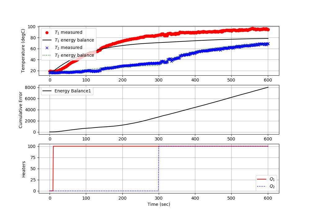
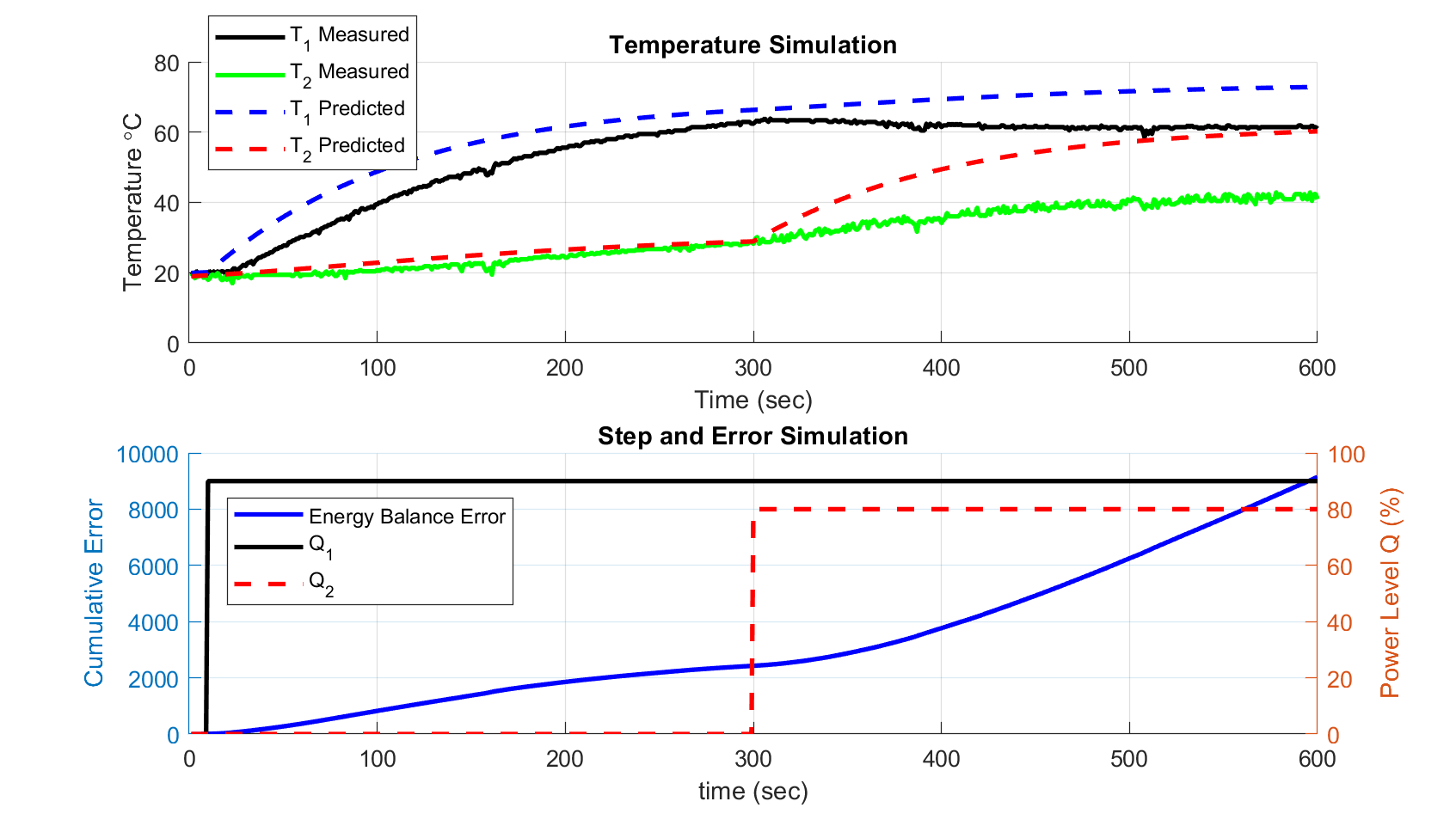
Test the agreement of the model with the Arduino temperature control lab. Report the cumulative error and the average error over 10 minutes with a step test for heater 1 at 10 seconds and heater 2 at 5 minutes.
Python
import numpy as np
import time
import matplotlib.pyplot as plt
from scipy.integrate import odeint
# define energy balance model
def heat(x,t,Q1,Q2):
# Parameters
Ta = 23 + 273.15 # K
U = 10.0 # W/m^2-K
m = 4.0/1000.0 # kg
Cp = 0.5 * 1000.0 # J/kg-K
A = 10.0 / 100.0**2 # Area in m^2
As = 2.0 / 100.0**2 # Area in m^2
alpha1 = 0.0100 # W / % heater 1
alpha2 = 0.0075 # W / % heater 2
eps = 0.9 # Emissivity
sigma = 5.67e-8 # Stefan-Boltzman
# Temperature States
T1 = x[0]
T2 = x[1]
# Heat Transfer Exchange Between 1 and 2
conv12 = U*As*(T2-T1)
rad12 = eps*sigma*As * (T2**4 - T1**4)
# Nonlinear Energy Balances
dT1dt = (1.0/(m*Cp))*(U*A*(Ta-T1) \
+ eps * sigma * A * (Ta**4 - T1**4) \
+ conv12 + rad12 \
+ alpha1*Q1)
dT2dt = (1.0/(m*Cp))*(U*A*(Ta-T2) \
+ eps * sigma * A * (Ta**4 - T2**4) \
- conv12 - rad12 \
+ alpha2*Q2)
return [dT1dt,dT2dt]
# save txt file
def save_txt(t,u1,u2,y1,y2,sp1,sp2):
data = np.vstack((t,u1,u2,y1,y2,sp1,sp2)) # vertical stack
data = data.T # transpose data
top = 'Time (sec), Heater 1 (%), Heater 2 (%), ' \
+ 'Temperature 1 (degC), Temperature 2 (degC), ' \
+ 'Set Point 1 (degC), Set Point 2 (degC)'
np.savetxt('data.txt',data,delimiter=',',header=top,comments='')
# Connect to Arduino
a = tclab.TCLab()
# Turn LED on
print('LED On')
a.LED(100)
# Run time in minutes
run_time = 10.0
# Number of cycles
loops = int(60.0*run_time)
tm = np.zeros(loops)
# Temperature (K)
Tsp1 = np.ones(loops) * 23.0 # set point (degC)
T1 = np.ones(loops) * a.T1 # measured T (degC)
Tsp2 = np.ones(loops) * 23.0 # set point (degC)
T2 = np.ones(loops) * a.T2 # measured T (degC)
# Predictions
Tp1 = np.ones(loops) * a.T1
Tp2 = np.ones(loops) * a.T2
error_eb = np.zeros(loops)
# impulse tests (0 - 100%)
Q1 = np.ones(loops) * 0.0
Q1[10:] = 100.0 # step up after 10 sec
Q2 = np.ones(loops) * 0.0
Q2[300:] = 100.0 # step up after 5 min (300 sec)
print('Running Main Loop. Ctrl-C to end.')
print(' Time Q1 Q2 T1 T2')
print('{:6.1f} {:6.2f} {:6.2f} {:6.2f} {:6.2f}'.format(tm[0], \
Q1[0], \
Q2[0], \
T1[0], \
T2[0]))
# Create plot
plt.figure(figsize=(10,7))
plt.ion()
plt.show()
# Main Loop
start_time = time.time()
prev_time = start_time
try:
for i in range(1,loops):
# Sleep time
sleep_max = 1.0
sleep = sleep_max - (time.time() - prev_time)
if sleep>=0.01:
time.sleep(sleep-0.01)
else:
time.sleep(0.01)
# Record time and change in time
t = time.time()
dt = t - prev_time
prev_time = t
tm[i] = t - start_time
# Read temperatures in Kelvin
T1[i] = a.T1
T2[i] = a.T2
# Simulate one time step with Energy Balance
Tinit = [Tp1[i-1]+273.15,Tp2[i-1]+273.15]
Tnext = odeint(heat,Tinit, \
[0,dt],args=(Q1[i-1],Q2[i-1]))
Tp1[i] = Tnext[1,0]-273.15
Tp2[i] = Tnext[1,1]-273.15
error_eb[i] = error_eb[i-1] \
+ (abs(Tp1[i]-T1[i]) \
+ abs(Tp2[i]-T2[i]))*dt
# Write output (0-100)
a.Q1(Q1[i])
a.Q2(Q2[i])
# Print line of data
print('{:6.1f} {:6.2f} {:6.2f} {:6.2f} {:6.2f}'.format(tm[i], \
Q1[i], \
Q2[i], \
T1[i], \
T2[i]))
# Plot
plt.clf()
ax=plt.subplot(3,1,1)
ax.grid()
plt.plot(tm[0:i],T1[0:i],'ro',label=r'$T_1$ measured')
plt.plot(tm[0:i],Tp1[0:i],'k-',label=r'$T_1$ energy balance')
plt.plot(tm[0:i],T2[0:i],'bx',label=r'$T_2$ measured')
plt.plot(tm[0:i],Tp2[0:i],'k--',label=r'$T_2$ energy balance')
plt.ylabel('Temperature (degC)')
plt.legend(loc=2)
ax=plt.subplot(3,1,2)
ax.grid()
plt.plot(tm[0:i],error_eb[0:i],'k-',label='Energy Balance Error')
plt.ylabel('Cumulative Error')
plt.legend(loc='best')
ax=plt.subplot(3,1,3)
ax.grid()
plt.plot(tm[0:i],Q1[0:i],'r-',label=r'$Q_1$')
plt.plot(tm[0:i],Q2[0:i],'b:',label=r'$Q_2$')
plt.ylabel('Heaters')
plt.xlabel('Time (sec)')
plt.legend(loc='best')
plt.draw()
plt.pause(0.05)
# Turn off heaters
a.Q1(0)
a.Q2(0)
# Save text file and plot at end
save_txt(tm[0:i],Q1[0:i],Q2[0:i],T1[0:i],T2[0:i],Tsp1[0:i],Tsp2[0:i])
# Save figure
plt.savefig('test_Models.png')
# Allow user to end loop with Ctrl-C
except KeyboardInterrupt:
# Disconnect from Arduino
a.Q1(0)
a.Q2(0)
print('Shutting down')
a.close()
save_txt(tm[0:i],Q1[0:i],Q2[0:i],T1[0:i],T2[0:i],Tsp1[0:i],Tsp2[0:i])
plt.savefig('test_Models.png')
# Make sure serial connection still closes when there's an error
except:
# Disconnect from Arduino
a.Q1(0)
a.Q2(0)
print('Error: Shutting down')
a.close()
save_txt(tm[0:i],Q1[0:i],Q2[0:i],T1[0:i],T2[0:i],Tsp1[0:i],Tsp2[0:i])
plt.savefig('test_Models.png')
raise
MATLAB

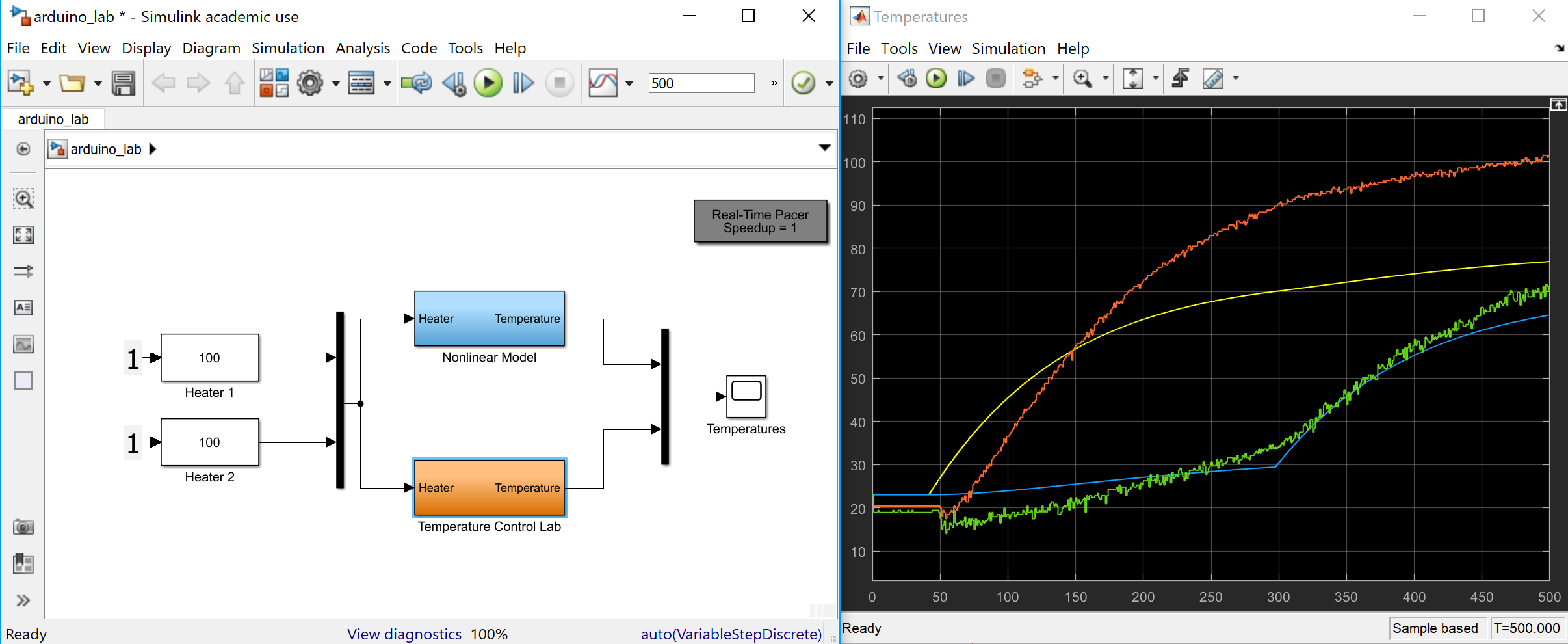
Simulink
Return to Temperature Control Lab Overview