Energy System Benchmark Problems
Optimized grid design and operation is needed as modern society depends on vast quantities of electrical energy. The complexity of the electric grid presents difficult control problems that require powerful solvers and efficient formulations for tractable solutions.


The Gekko Optimization Suite is a machine learning and optimization package in Python for mixed-integer and differential algebraic equations and is capable of solving complex grid design and control problems.

A series of non-dimensional benchmark cases are proposed for grid energy production. These include:
Individual case studies include ramp rate constraints, power production, and energy storage operation as design variables. Variables used in the benchmark problems are defined below.
| Symbol | Description |
| `J` | objective function |
| d | demand |
| g | generation |
| r | ramp rate |
| e | storage inventory |
| ein, eout | energy stored, recovered |
| R | renewable source |
| sin, sout | slack variables for storage switching |
| `\eta` | storage efficiency |
| n | number of generating units |
| i | subscript indicates product i |
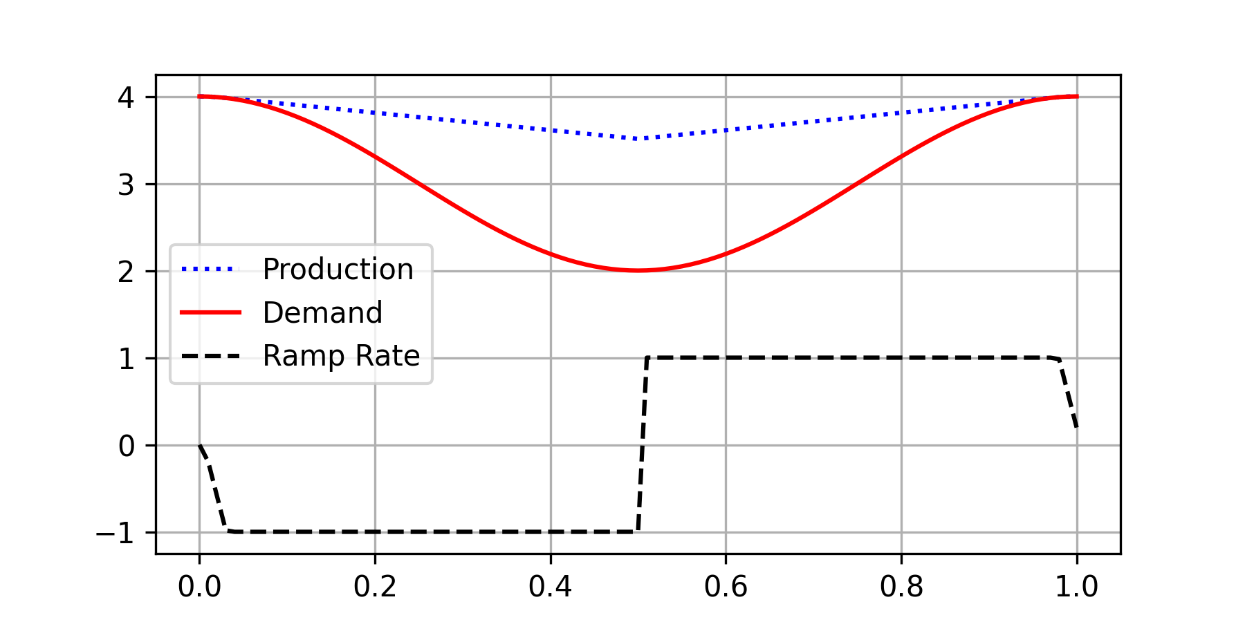
Benchmark I: Load Following
The first benchmark problem represents load following, a common scenario in grid systems. The optimizer seeks to match demand and supply with fluctuating demand dynamics. A single generator with ramping constraints attempts to respond to a single load with perfect foresight. The generation and demand match initially, but the generator must ramp in order to ensure this throughout the horizon while minimizing overproduction.
$$ \begin{align} \min_{r} \ & J = \int_{t=0}^{1} \left [ 1000 \max(0, d - g) + \max(0, g - d) \right ]dt \\ \mathrm{s.t.}\ & \frac{dg}{dt} = r \\ & d=\cos\left({2\pi t}\right) + 3 \label{eqn:benchmark1c}\\ & -1 \leq r \leq 1 \label{eqn:benchmark1d}\\ & g(0)=d(0)=4 \end{align} $$
import numpy as np
import matplotlib.pyplot as plt
t = np.linspace(0,1,101)
m = GEKKO(remote=False); m.time=t
d = m.Param(np.cos(2*np.pi*t)+3)
g = m.Var(d[0])
J = m.CV(0)
J.STATUS=1; J.SPHI=J.SPLO=0
J.WSPHI=1000; J.WSPLO=1
r = m.MV(0,lb=-1,ub=1); r.STATUS=1
m.Equations([g.dt()==r, J==d-g])
m.options.IMODE=6; m.solve()
plt.plot(t,g,'b:',label='Production')
plt.plot(t,d,'r-',label='Demand')
plt.plot(t,r,'k--',label='Ramp Rate')
plt.legend(); plt.grid(); plt.show()
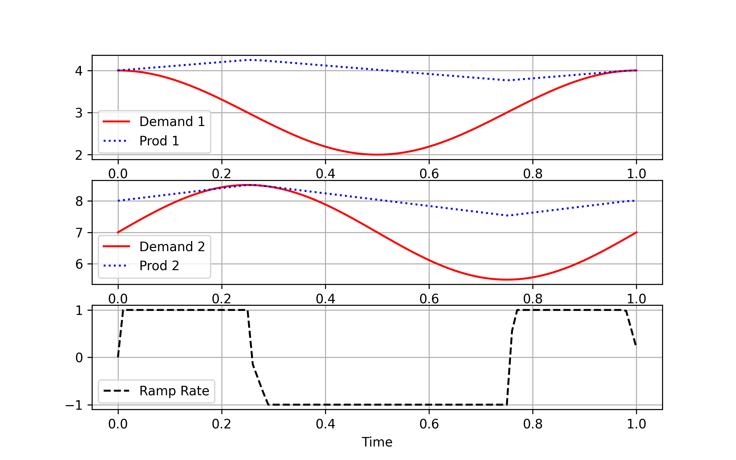
Benchmark II: Cogeneration
In the second benchmark problem, one producer seeks to meet two objectives that are constraining at different times. Benchmark II enhances Benchmark I by replacing the generator with a cogeneration system n=2 that produces (1) electricity and (2) heat in response to electricity demand and a new heat demand profile, again with perfect foresight.
$$ \begin{align} \min_{r} \ \ & J = \sum_{i=1}^n \int_{t=0}^{1} \, \left [ 1000 \; \max(0, \, d_i - g_i) \vphantom{\int} + \max(0, \, g_i - d_i) \vphantom{\int} \right ]dt \\ \mathrm{s.t.}\ \ & \frac{dg_1}{dt} = r, \enspace g_2 = 2 g_1 \label{eqn:benchmark2b}\\ & d_1=\cos\left({2\pi t}\right) + 3 \\ & d_2=1.5\sin\left({2\pi t}\right) + 7 \\ & -1 \leq r \leq 1 \\ & g_1(0)=d_1(0)=4 \\ & g_2(0)=8, \; d_2(0)=7 \end{align} $$
import numpy as np
import matplotlib.pyplot as plt
t = np.linspace(0,1,101)
m = GEKKO(remote=False); m.time=t
d1 = m.Param(np.cos(2*np.pi*t)+3)
d2 = m.Param(1.5*np.sin(2*np.pi*t)+7)
g1 = m.Var(d1[0]); g2 = m.Intermediate(g1*2)
J1 = m.CV(0); J1.STATUS=1; J1.SPHI=J1.SPLO=0; J1.WSPHI=1000; J1.WSPLO=1
J2 = m.CV(0); J2.STATUS=1; J2.SPHI=J2.SPLO=0; J2.WSPHI=1000; J2.WSPLO=1
r = m.MV(0,lb=-1,ub=1); r.STATUS=1
m.Equations([g1.dt()==r, J1==d1-g1, J2==d2-g2])
m.options.IMODE=6; m.solve()
plt.figure(figsize=(8,5))
plt.subplot(3,1,1)
plt.plot(t,d1,'r-',label='Demand 1')
plt.plot(t,g1,'b:',label='Prod 1')
plt.grid(); plt.legend()
plt.subplot(3,1,2)
plt.plot(t,d2,'r-',label='Demand 2')
plt.plot(t,g2,'b:',label='Prod 2')
plt.grid(); plt.legend()
plt.subplot(3,1,3)
plt.plot(t,r,'k--',label='Ramp Rate')
plt.grid(); plt.legend(); plt.xlabel('Time')
plt.show()
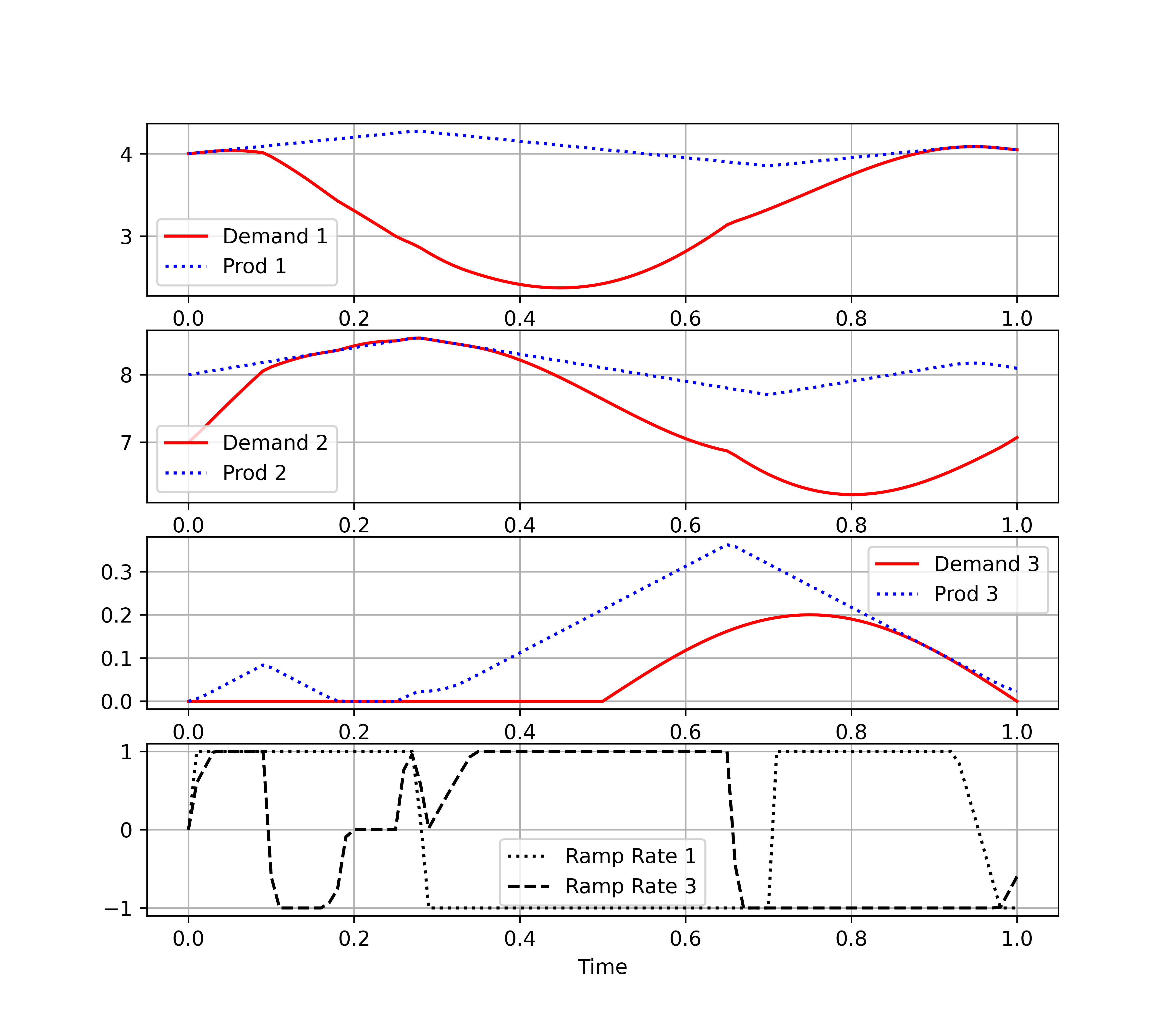
Benchmark III: Tri-generation
The third benchmark problem enhances the previous problems further still, creating a tri-generation system n=3 with two producers, three products, and three demand profiles. The primary producer is the same as the prior benchmark and is ramp-rate constrained to produce the two primary products (e.g., electricity and heat). An additional producer (e.g., a solid oxide electrolysis cell) uses these first two products to make a third product (e.g., hydrogen), thereby utilizing any excess system capacity and maximizing its production while avoiding supply shortages for products one and two. As before, the optimizer has perfect foresight.
$$ \begin{align} \min_{r_1, r_3} \ \ & J = \sum_{i=1}^n \int_{t=0}^{1} \left [ \vphantom{\int} 1000 \; \max(0, \, d_i - g_i) + \max(0, \, g_i - d_i) \vphantom{\int} \right ]dt - 0.1 \int_{t=0}^{1} g_3 dt \\ \mathrm{s.t.}\ \ & \frac{dg_1}{dt} = r_1, \; \frac{dg_3}{dt} = r_3 \\ & g_2 = 2 g_1 \\ & d_1=\cos\left({2\pi t}\right) + 3 + 2 g_3 \\ & d_2=1.5\sin\left({2\pi t}\right) + 7 + 3 g_3 \\ & d_3=\max\left[0,-0.2\sin\left(2\pi t\right) \right] \\ & -1 \leq r_1 \leq 1, \enspace -1 \leq r_3 \leq 1 \\ & g_1(0)=d_1(0)=4 \\ & g_2(0)=8, \; d_2(0)=7 \\ & g_3(0)=d_3(0)=0 \end{align} $$
from gekko import GEKKO
import matplotlib.pyplot as plt
t = np.linspace(0,1,101)
m = GEKKO(remote=False); m.time=t
d1 = m.Param(np.cos(2*np.pi*t)+3)
d2 = m.Param(1.5*np.sin(2*np.pi*t)+7)
d3 = m.Param(np.clip(-0.2*np.sin(2*np.pi*t),0,None))
d1v = m.Var(d1[0]); d2v=m.Intermediate(d1v*2)
d3v = m.Var(0,lb=0); d3v1=m.Var(0); d3v2=m.Var(0)
t1 = m.Intermediate(d1+d3v1); t2 = m.Intermediate(d2+d3v2)
e = m.CV(0); e.STATUS=1; e.SPHI=e.SPLO=0; e.WSPHI=1000; e.WSPLO=1
h = m.CV(0); h.STATUS=1; h.SPHI=h.SPLO=0; h.WSPHI=1000; h.WSPLO=1
z = m.CV(0); z.STATUS=1; z.SPHI=z.SPLO=0; z.WSPHI=1000; z.WSPLO=1
r1 = m.MV(0,lb=-1,ub=1); r1.STATUS=1; r1.DCOST=0.0
r3 = m.MV(0,lb=-1,ub=1); r3.STATUS=1; r3.DCOST=0.0
m.Equations([d1v.dt()==r1, e==t1-d1v, h==t2-d2v])
m.Equations([d3v.dt()==r3, z==d3-d3v, d3v1==d3v*2, d3v2==d3v*3])
m.Maximize(d3v)
m.options.IMODE=6; m.options.SOLVER=1; m.solve()
plt.figure(figsize=(8,7))
plt.subplot(4,1,1)
plt.plot(t,t1,'r-',label='Demand 1')
plt.plot(t,d1v,'b:',label='Prod 1')
plt.legend(); plt.grid()
plt.subplot(4,1,2)
plt.plot(t,t2,'r-',label='Demand 2')
plt.plot(t,d2v,'b:',label='Prod 2')
plt.legend(); plt.grid()
plt.subplot(4,1,3)
plt.plot(t,d3,'r-',label='Demand 3')
plt.plot(t,d3v,'b:',label='Prod 3')
plt.legend(); plt.grid()
plt.subplot(4,1,4)
plt.plot(t,r1,'k:',label='Ramp Rate 1')
plt.plot(t,r3,'k--',label='Ramp Rate 3')
plt.legend(); plt.grid(); plt.xlabel('Time')
plt.show()
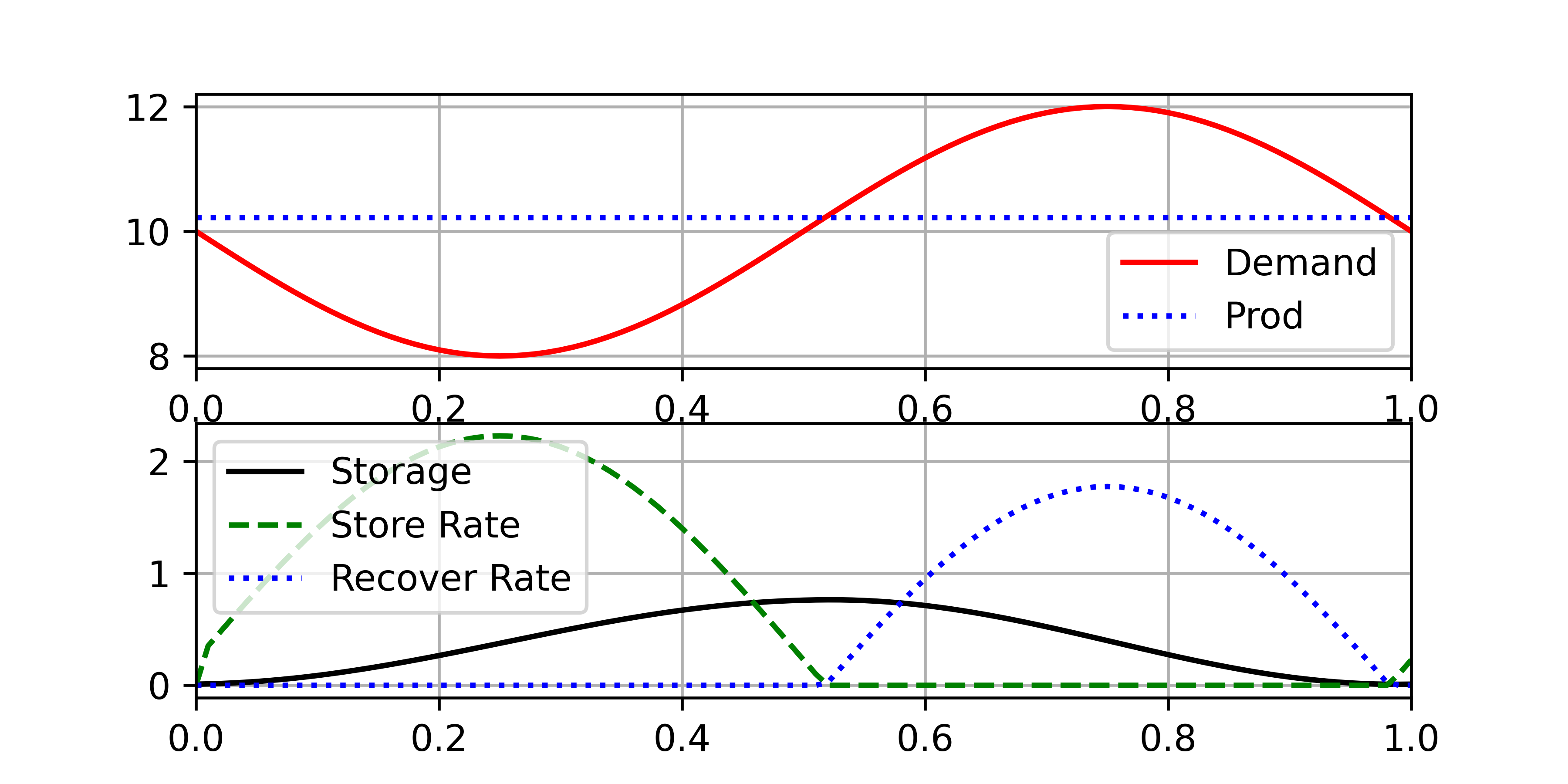
Benchmark IV: Constant Production with Storage
The fourth benchmark problem models a hybrid system with a single generator with constant production constraints coupled with energy storage that together must meet an oscillating electricity demand. The goal of the problem is to minimize the required power production and use energy storage to capture excess generation serve the oscillating energy demand while keeping the base-load generator production constant. As before, the model has perfect foresight. In order to prevent the energy storage from charging and discharging simultaneously without requiring mixed-integer variables, slack variables are used to control when the storage charges and discharges, allowing it to switch modes in a way that is both continuous and differentiable. This allows the modeling language to use automatic differentiation to provide exact gradients to the solver.
$$ \begin{align} \min_g \ \ & g \\ \mathrm{s.t.} & \frac{de}{dt} = e_{\text{in}} - e_{\text{out}} \cdot \eta \\ & e_{\text{in}} = g - d + s_{\text{in}} \\ & e_{\text{out}} = d - g + s_{\text{out}} \\ & g - d = s_{\text{out}} - s_{\text{in}} \\ & s_{\text{out}}, \, s_{\text{in}} \geq 0, \enspace e_{\text{out}} \cdot e_{\text{in}} \leq 0 \\ & g + e_{\text{out}}/\eta - e_{\text{in}} \geq d \\ & e \geq 0, \enspace \eta = 0.7 \\ & d = 10 - 2 \sin(2 \, \pi \, t) \\ & e(0) = e(1) = 0 \end{align} $$
import numpy as np
import matplotlib.pyplot as plt
m = GEKKO(remote=False)
m.time = np.linspace(0,1,101)
g = m.FV(); g.STATUS = 1 # production
s = m.Var(1e-2, lb=0) # storage inventory
store = m.Var() # store energy rate
s_in = m.Var(lb=0) # store slack variable
recover = m.Var() # recover energy rate
s_out = m.Var(lb=0) # recover slack variable
eta = 0.7
d = m.Param(-2*np.sin(2*np.pi*m.time)+10)
m.periodic(s)
m.Equations([g + recover/eta - store >= d,
g - d == s_out - s_in,
store == g - d + s_in,
recover == d - g + s_out,
s.dt() == store - recover/eta,
store * recover <= 0])
m.Minimize(g)
m.options.SOLVER = 1
m.options.IMODE = 6
m.options.NODES = 3
m.solve()
plt.figure(figsize=(6,3))
plt.subplot(2,1,1)
plt.plot(m.time,d,'r-',label='Demand')
plt.plot(m.time,g,'b:',label='Prod')
plt.legend(); plt.grid(); plt.xlim([0,1])
plt.subplot(2,1,2)
plt.plot(m.time,s,'k-',label='Storage')
plt.plot(m.time,store,'g--', label='Store Rate')
plt.plot(m.time,recover,'b:', label='Recover Rate')
plt.legend(); plt.grid(); plt.xlim([0,1])
plt.show()
Benchmark V: Load Following with Storage
The fifth benchmark combines energy storage with a load-following problem similar to Benchmark I. The first-half of the time horizon is nearly identical to Benchmark I, but now the excess energy can be stored. This allows the system to meet a higher demand in the second half of the time horizon without needing extremes in generation. The solver minimizes the ramping needs and operates more flexibly by storing and then recovering the overproduction caused by the ramping constraints. Energy storage allows this generator to meet the load without requiring significant overproduction.
$$ \begin{align} \min_{r} \ \ & J = \sum_{i=1}^n \int_{t=0}^{1} \, [ 1000 \, \max(0, \, \Psi) \vphantom{\int} + \, \max(0, \, -\Psi) \vphantom{\int} ]dt \\ & \text{where} \ \Psi = d - g - R + e_{\text{out}}/\eta - e_{\text{in}} \\ \mathrm{s.t.}\ \ & \frac{de}{dt} = e_{\text{in}} - e_{\text{out}} \cdot \eta \\ & e_{\text{in}} = g + R - d + s_{\text{in}} \\ & e_{\text{out}} = d - g - R + s_{\text{out}} \\ & g + R - d = s_{\text{out}} - s_{\text{in}} \\ & s_{\text{out}}, \, s_{\text{in}} \geq 0, \enspace e_{\text{out}} \cdot e_{\text{in}} \leq 0\\ & g + R + e_{\text{out}}/\eta - e_{\text{in}} \geq d \\ & e \geq 0, \enspace \eta = 0.85 \\ & d = 7 - 2 \sin(2 \, \pi \, t) \\ & R = \begin{cases} 3 + 3 \cos(4 \, \pi \, t) & \frac{1}{4} \leq t \leq \frac{3}{4} \\ 0 & \mbox{otherwise} \\ \end{cases} \\ & \frac{dg}{dt} = r, \enspace -1\leq r \leq 1 \\ & e(0) = e(1) = 0 \end{align} $$
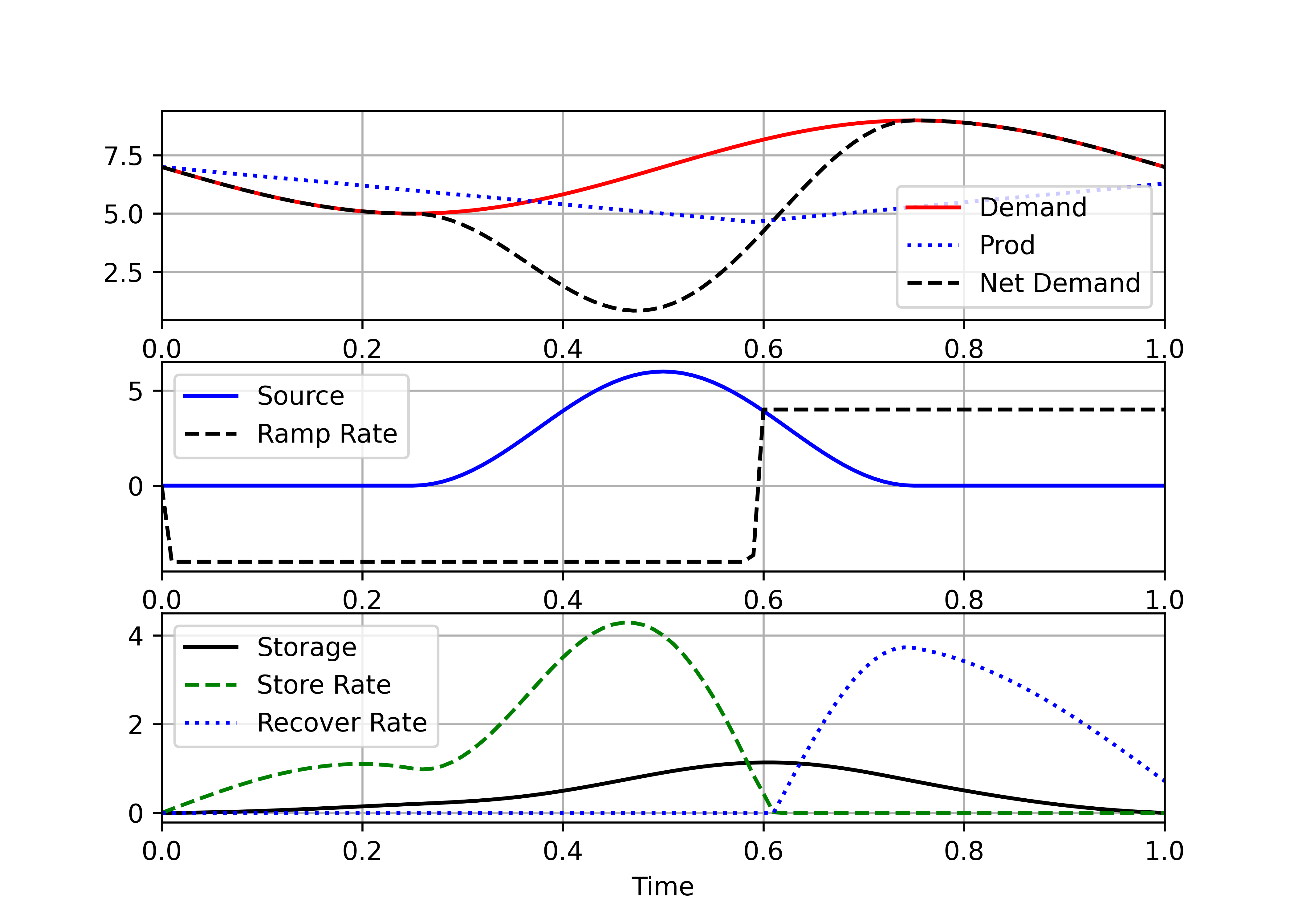
import numpy as np
import matplotlib.pyplot as plt
m = GEKKO(remote=False)
m.time = np.linspace(0,1,101)
# renewable energy source
renewable = 3*np.cos(np.pi*m.time/6*24)+3
num = len(m.time)
center = np.ones(num)
center[0:int(num/4)] = 0
center[-int(num/4):] = 0
renewable *= center
r = m.Param(renewable)
dg = m.MV(0, lb=-4, ub=4); dg.STATUS = 1
d = m.Param(-2*np.sin(2*np.pi*m.time)+7)
net = m.Intermediate(d-r)
g = m.Var(d[0]) # production
s = m.Var(0, lb=0) # storage inventory
store = m.Var() # store energy rate
s_in = m.Var(lb=0) # store slack variable
recover = m.Var() # recover energy rate
s_out = m.Var(lb=0) # recover slack variable
m.periodic(s)
eta = 0.85 # storage efficiency
m.Minimize(g)
err = m.CV(0); err.STATUS = 1
err.SPHI = err.SPLO = 0
err.WSPHI = 1000; err.WSPLO = 1
m.Minimize(0.01*err**2)
m.Equations([g.dt() == dg,
err == d - g - r + recover/eta - store,
g + r - d == s_out - s_in,
store == g + r - d + s_in,
recover == d - g - r + s_out,
s.dt() == store - recover/eta,
store * recover <= 0])
m.options.SOLVER = 1
m.options.IMODE = 6
m.options.NODES = 2
m.solve()
plt.figure(figsize=(7,5))
plt.subplot(3,1,1)
plt.plot(m.time,d,'r-',label='Demand')
plt.plot(m.time,g,'b:',label='Prod')
plt.plot(m.time,net,'k--',label='Net Demand')
plt.legend(); plt.grid(); plt.xlim([0,1])
plt.subplot(3,1,2)
plt.plot(m.time,r,'b-',label='Source')
plt.plot(m.time,dg,'k--',label='Ramp Rate')
plt.legend(); plt.grid(); plt.xlim([0,1])
plt.subplot(3,1,3)
plt.plot(m.time,s,'k-',label='Storage')
plt.plot(m.time,store,'g--', label='Store Rate')
plt.plot(m.time,recover,'b:', label='Recover Rate')
plt.xlim([0,1]); plt.xlabel('Time')
plt.legend(); plt.grid()
plt.show()
Benchmark VI: Cogeneration with Dual Storage
The sixth benchmark problem is a combination of Benchmarks II and V where the ramp rate of the generator is the manipulated variable but now must meet both electrical (1) and heat (2) demand with the use of both electrical and thermal storage. A renewable generation source (such as solar PV) is added to the system as an auxiliary electrical energy source that cannot be controlled. The objective is the same as in Benchmark IV, to minimize power production, but this time while meeting both the heat and power demands. The model again has perfect foresight. Slack variables are used in the same way as in Benchmarks IV and V.
$$ \begin{align} \min_{r_1} \ \ & g_1 \\ \mathrm{s.t.}\ \ & \frac{de_i}{dt} = e_{\text{in},i} - e_{\text{out},i}\cdot \eta_i \\ & e_{\text{in},i} = g_i + R_i - d_i + s_{\text{in},i} \\ & e_{\text{out},i} = d_i - g_i - R_i + s_{\text{out},i} \\ & g_i + R_i - d_i = s_{\text{out},i} - s_{\text{in},i} \\ & s_{\text{out},i}, \, s_{\text{in},i} \geq 0, \enspace e_{\text{out},i} \cdot e_{\text{in},i} \leq 0 \\ & g_i + R_i + e_{\text{out},i}/\eta_i - e_{\text{in},i} \geq d_i \\ & e_i \geq 0, \enspace \eta_1 = 0.7, \enspace \eta_2 = 0.8 \\ & d_1 = 10 - 2 \sin(2 \, \pi \, t) \\ & d_2 = 15 + 1.5 \cos(2 \, \pi \, t) \\ & R_1 = \begin{cases} 2 + 2 \cos(4 \, \pi \, t) & \frac{1}{4} \leq t \leq \frac{3}{4} \\ 0 & \mbox{otherwise} \\ \end{cases} \\ & \frac{dg_1}{dt} = r_1, \enspace -3\leq r_1 \leq 3 \\ & R_2 = 0, \enspace g_2 = 1.5 \cdot g_1 \\ & e_1(0) = 0, \enspace e_2(0) = e_2(1) = 0.5 \end{align} $$
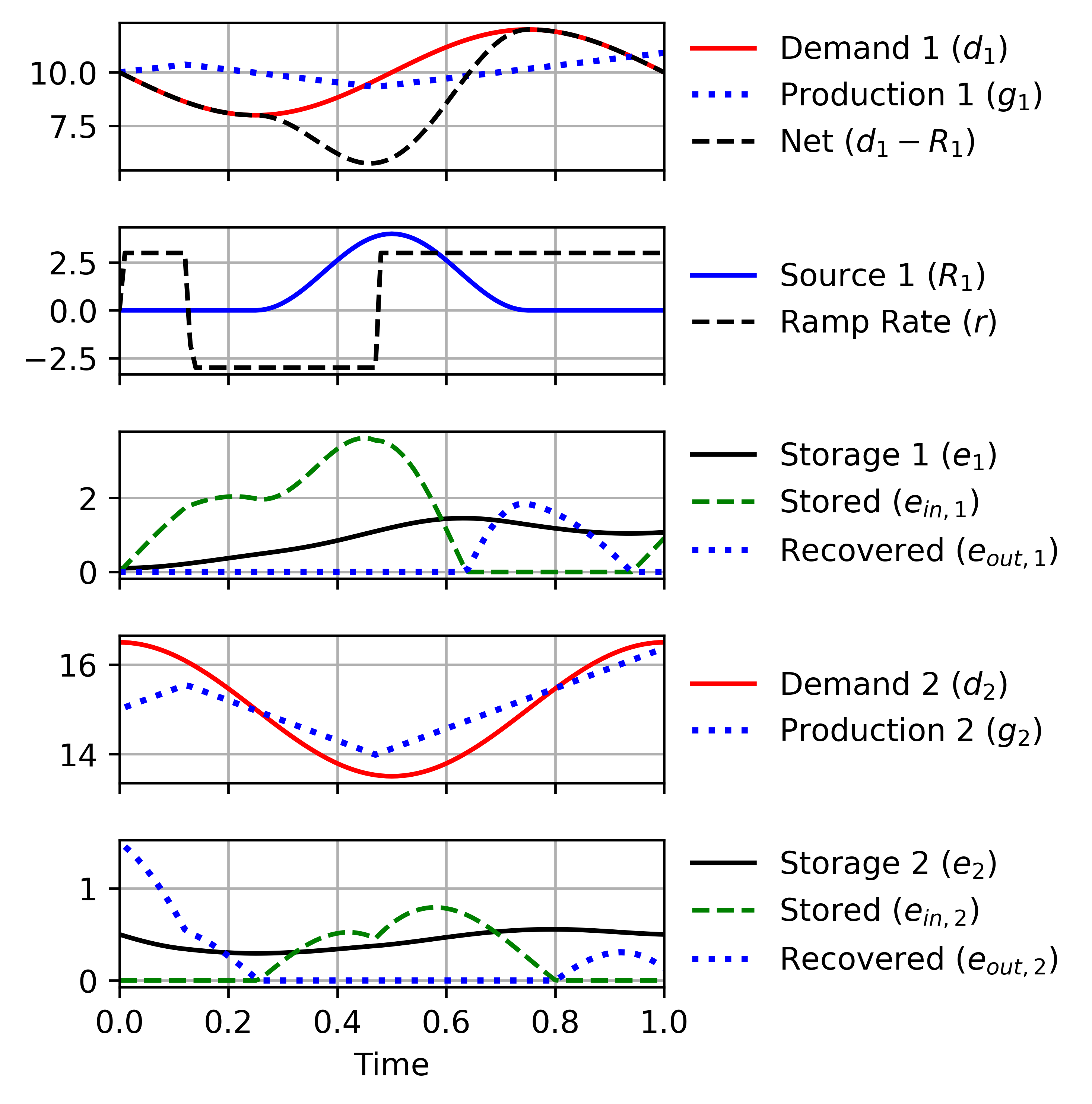
import numpy as np
import matplotlib.pyplot as plt
m = GEKKO(remote=False)
t = np.linspace(0, 1, 101)
m.time = t
m.options.SOLVER = 3
m.options.IMODE = 6
m.options.NODES = 2
m.options.CV_TYPE = 1
m.options.MAX_ITER = 1000
p = m.SV(10) # production (constant)
s = m.Var(0.1, lb=0) # storage inventory
stored = m.SV() # store energy rate
recovery = m.SV() # recover energy rate
vx = m.SV(lb=0) # recover slack variable
vy = m.SV(lb=0) # store slack variable
eps = 0.85 # Storage efficiency
d = m.MV((-20*np.sin(np.pi*t/12*24)+100)/10)
d_h = m.MV((15*np.cos(np.pi*t/12*24)+150)/10)
p_h_initial = m.Intermediate(p*1.5)
p_h = m.SV(p_h_initial)
s_h = m.Var(0.5,lb=0)
stored_h = m.SV()
recovery_h = m.SV()
#renewable energy source
renewable = (20*np.cos(np.pi*t/6*24)+20)/10
center = np.ones(len(t))
num = len(t)
center[0:int(num/4)] = 0
center[-int(num/4):] = 0
renewable *= center
r = m.Param(renewable)
r1 = m.MV(ub=3,lb=-3)
r1.STATUS=1
m.periodic(s_h)
zx = m.SV(lb=0)
zy = m.SV(lb=0)
eps_h = 0.8 # heat storage efficiency
net = m.Intermediate(d-r)
m.Equations([p + r + recovery/eps - stored >= d,
p + r - d == vx - vy,
stored == p + r - d + vy,
recovery == d - p - r + vx,
s.dt() == stored - recovery/eps,
p.dt() == r1,
stored * recovery <= 0,
p_h + recovery_h/eps_h - stored_h >= d_h,
p_h - d_h == zx - zy,
stored_h == p_h - d_h + zy,
recovery_h == d_h - p_h + zx,
s_h.dt() == stored_h - recovery_h/eps_h,
stored_h * recovery_h <= 0,
p_h == 1.5 * p])
m.Minimize(p)
m.solve()
# Plot solution
fig, axes = plt.subplots(5, 1, figsize=(5, 5.1), sharex=True)
axes = axes.ravel()
ax = axes[0]
ax.plot(t, d, 'r-', label='Demand 1 ($d_1$)')
ax.plot(t, p,'b:', label='Production 1 ($g_1$)',lw=2)
ax.plot(t, net, 'k--', label='Net ($d_1-R_1$)')
ax = axes[1]
ax.plot(t,r, 'b-',label='Source 1 ($R_1$)')
ax.plot(t,r1, 'k--', label='Ramp Rate ($r$)')
ax = axes[2]
ax.plot(t,s, 'k-', label='Storage 1 ($e_1$)')
ax.plot(t,stored,'g--',label='Stored ($e_{\text{in},1}$)')
ax.plot(t,recovery,'b:',label='Recovered ($e_{\text{out},1}$)',lw=2)
ax = axes[3]
ax.plot(t,d_h, 'r-', label='Demand 2 ($d_2$)')
ax.plot(t[1:], p_h.value[1:],'b:',\
label='Production 2 ($g_2$)',lw=2)
ax = axes[4]
ax.plot(t,s_h, 'k-', label='Storage 2 ($e_2$)')
ax.plot(t,stored_h,'g--',label='Stored ($e_{\text{in},2}$)')
ax.plot(t[1:],recovery_h.value[1:],'b:',\
label='Recovered ($e_{\text{out},2}$)',lw=2)
ax.set_xlabel('Time')
for ax in axes:
ax.legend(loc='center left',\
bbox_to_anchor=(1,0.5),frameon=False)
ax.grid()
ax.set_xlim(0, 1)
plt.tight_layout()
plt.savefig('grid_energy6.png', dpi=600,\
bbox_inches = 'tight')
plt.show()
Reference

Gates, N.S., Hill, D.C., Billings, B.W., Powell, K.M., Hedengren, J.D., Benchmarks for Grid Energy Management with Python Gekko, 60th IEEE Conference on Decision and Control (CDC), Tutorial Session: Open Source Software for Control Applications, Austin, TX, Dec 13-15, 2021. Preprint
Acknowledgement
Financial support from the Department of Energy Nuclear Energy University Program Grant Number DE-NE0008866.