OCP Benchmarks
Optimal Control Problem (OCP) solvers are a powerful tool for designing control strategies that optimize a given objective function subject to constraints. They are widely used in engineering, economics, finance, and management, and are applied to a wide range of problems to find optimal solutions that minimize costs, maximize profits, reduce risk, or achieve other desired outcomes. The control strategy is typically represented as a function of time that maps the control input (manipulated variable) to the state of the system. The state of the system is determined by a set of differential equations, and the objective function is a measure of the system performance over a time horizon.
Exercise
Objective: Set up and solve several OCP benchmarks. Create a program to optimize and display the results. Estimated Time (each): 30 minutes
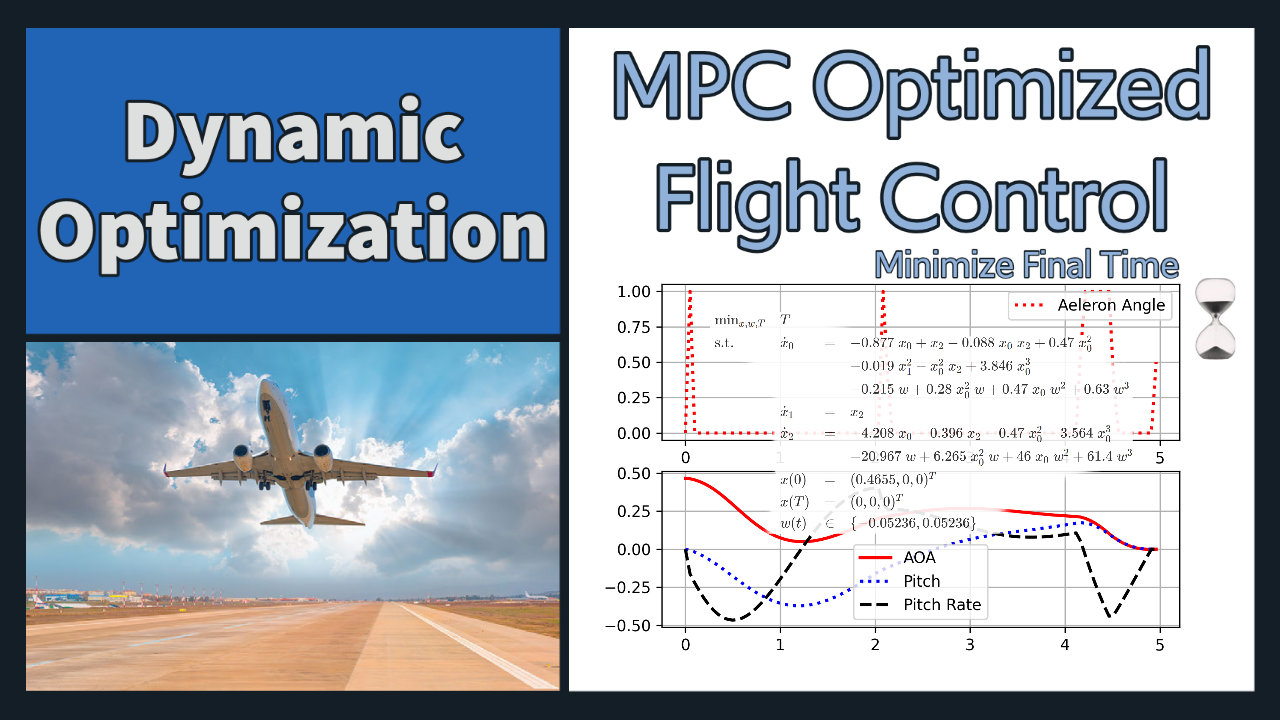
Aircraft Control
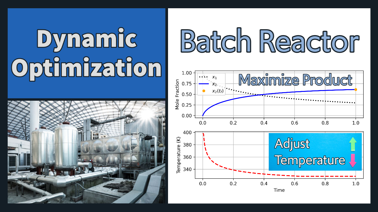
Batch Reactor
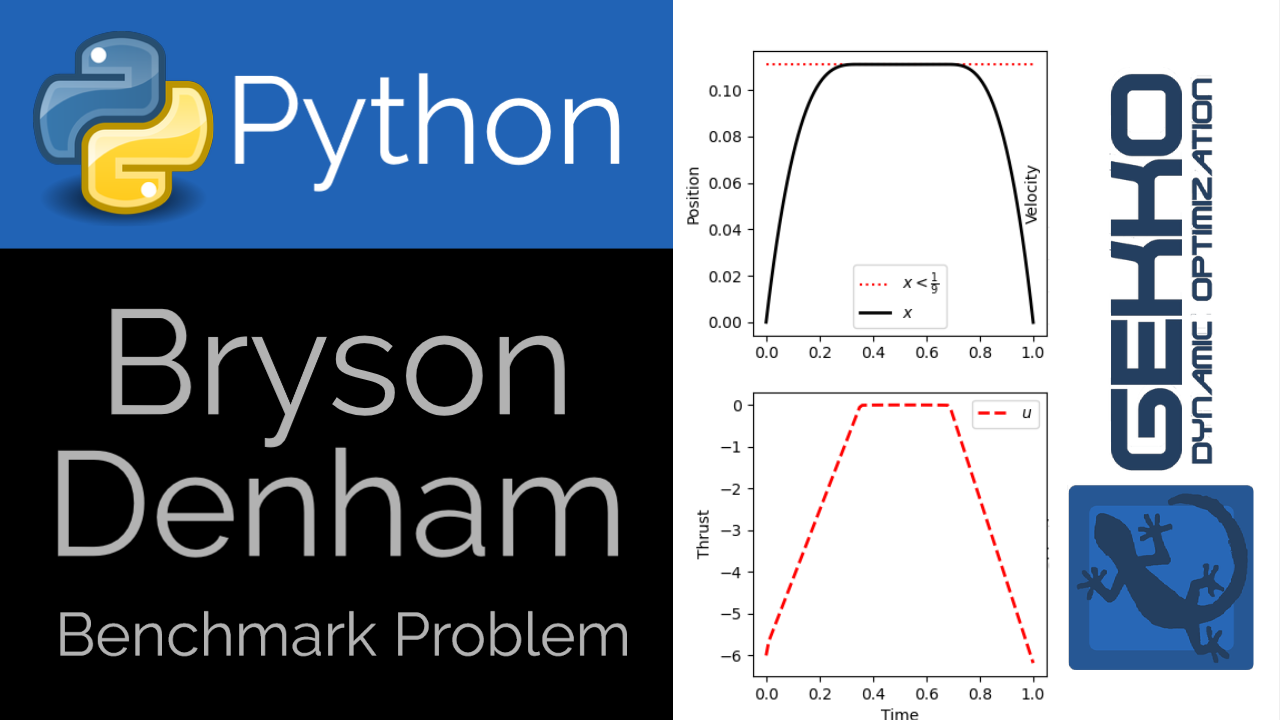
Bryson-Denham Problem
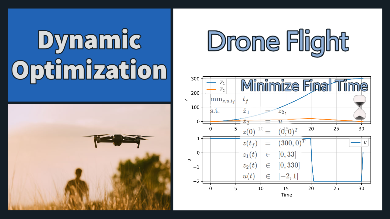
Drone Flight
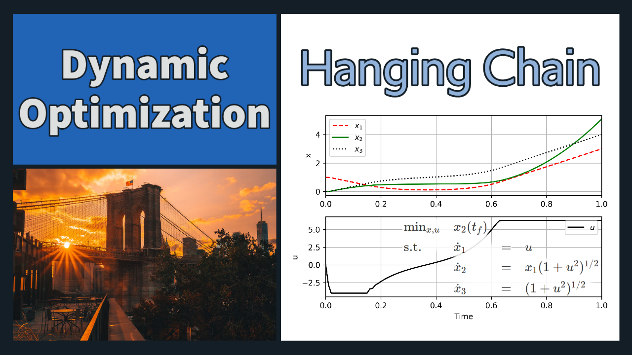
Hanging Chain
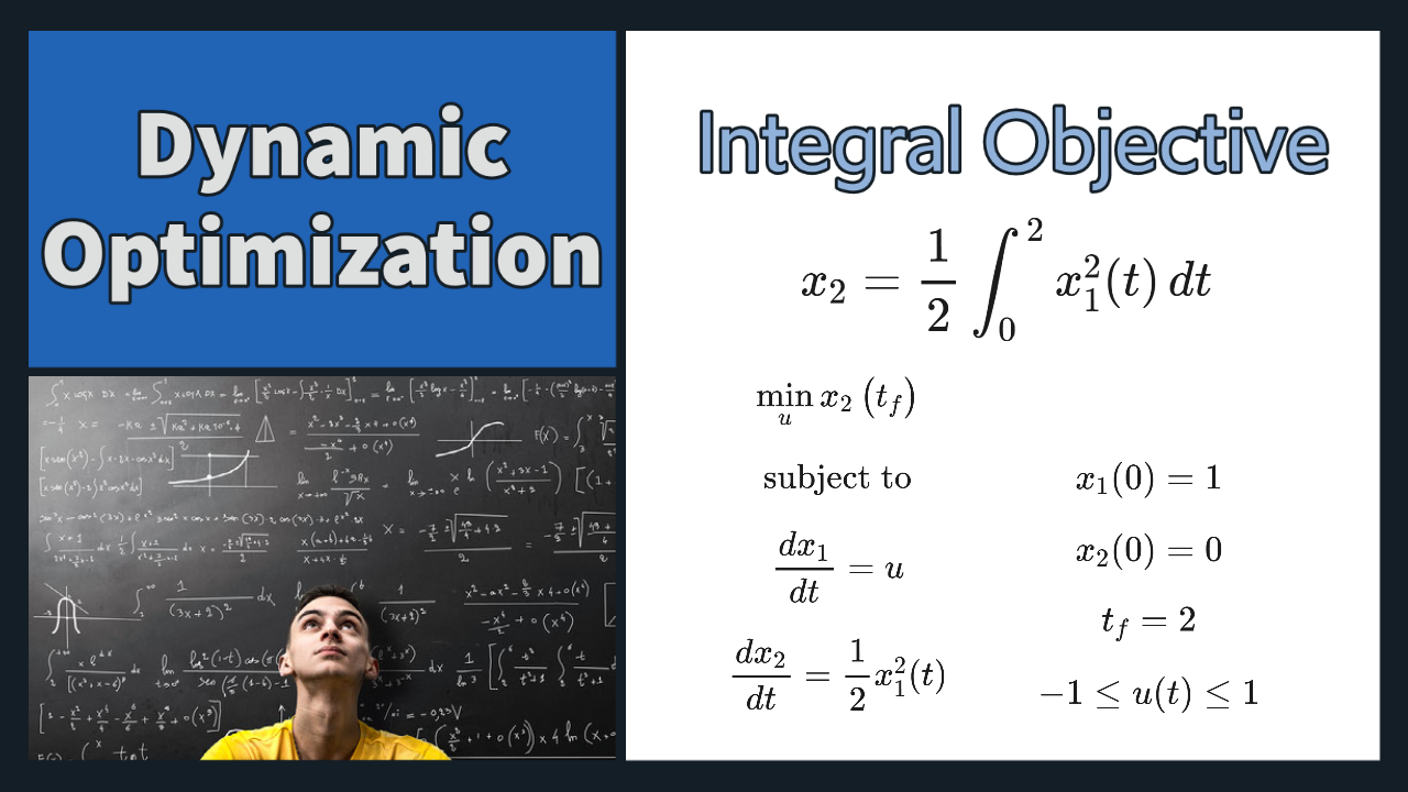
Integral Objective (Luus)
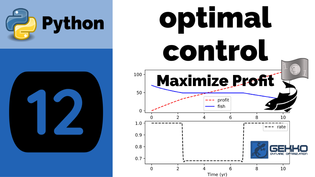
Maximize Profit (Commercial Fishery)
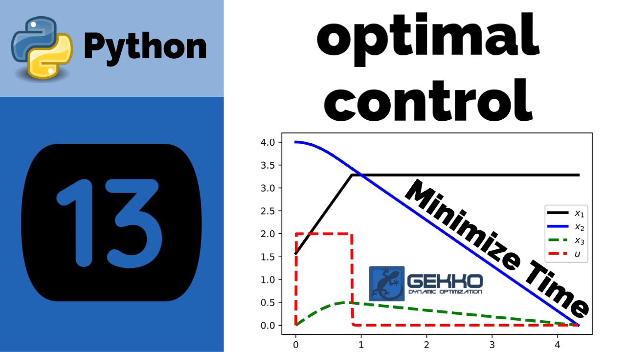
Minimize Final Time (Jennings)
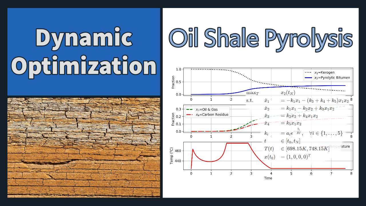
Oil Shale Pyrolysis
Electric Vehicle Energy

Aly-Chan Singular Control Problem
- Solve the following nonlinear and constrained problem.
- The objective is to minimize final state x3(pi/2) by adjusting the value of u.
- Compare to the exact solution of u(t)= -sin(t).

import matplotlib.pyplot as plt
from gekko import GEKKO
m = GEKKO()
nt = 1001
t = np.linspace(0,np.pi/2,nt)
m.time = t
# Variables
x1 = m.Var(value=0)
x2 = m.Var(value=1)
x3 = m.Var(value=0)
u = m.MV(value=0,ub=1,lb=-1)
u.STATUS = 1
u.DCOST = 0
p = np.zeros(nt)
p[-1] = 1.0
final = m.Param(value=p)
# Equations
m.Equation(x1.dt()==x2)
m.Equation(x2.dt()==u)
m.Equation(2*x3.dt()==x2**2-x1**2)
# Objective Function
m.Obj(x3*final)
m.options.IMODE = 6
m.options.NODES = 4
m.solve()
plt.figure(1)
plt.subplot(2,1,1)
plt.plot(m.time,x1.value,'k:',lw=2,label=r'$x_1$')
plt.plot(m.time,x2.value,'b-',lw=2,label=r'$x_2$')
plt.plot(m.time,x2.value,'k-',lw=2,label=r'$x_3$')
plt.subplot(2,1,2)
plt.plot(m.time,u.value,'r--',lw=2,label=r'$u$')
plt.plot(t,-np.sin(t),'k:',lw=2,label='Exact')
plt.legend(loc='best')
plt.xlabel('Time')
plt.ylabel('Value')
plt.show()
Aly Singular Control Problem
See estimation example using the same model to explain estimator objectives.
Catalyzed Reaction
References
- Beal, L.D.R., Hill, D., Martin, R.A., and Hedengren, J. D., GEKKO Optimization Suite, Processes, Volume 6, Number 8, 2018, doi: 10.3390/pr6080106. Article
- Hedengren, J. D. and Asgharzadeh Shishavan, R., Powell, K.M., and Edgar, T.F., Nonlinear Modeling, Estimation and Predictive Control in APMonitor, Computers and Chemical Engineering, Volume 70, pg. 133–148, 2014. Article
- Aly G.M. and Chan W.C. Application of a modified quasilinearization technique to totally singular optimal problems. International Journal of Control, 17(4): 809-815, 1973.