Hanging Chain Optimization
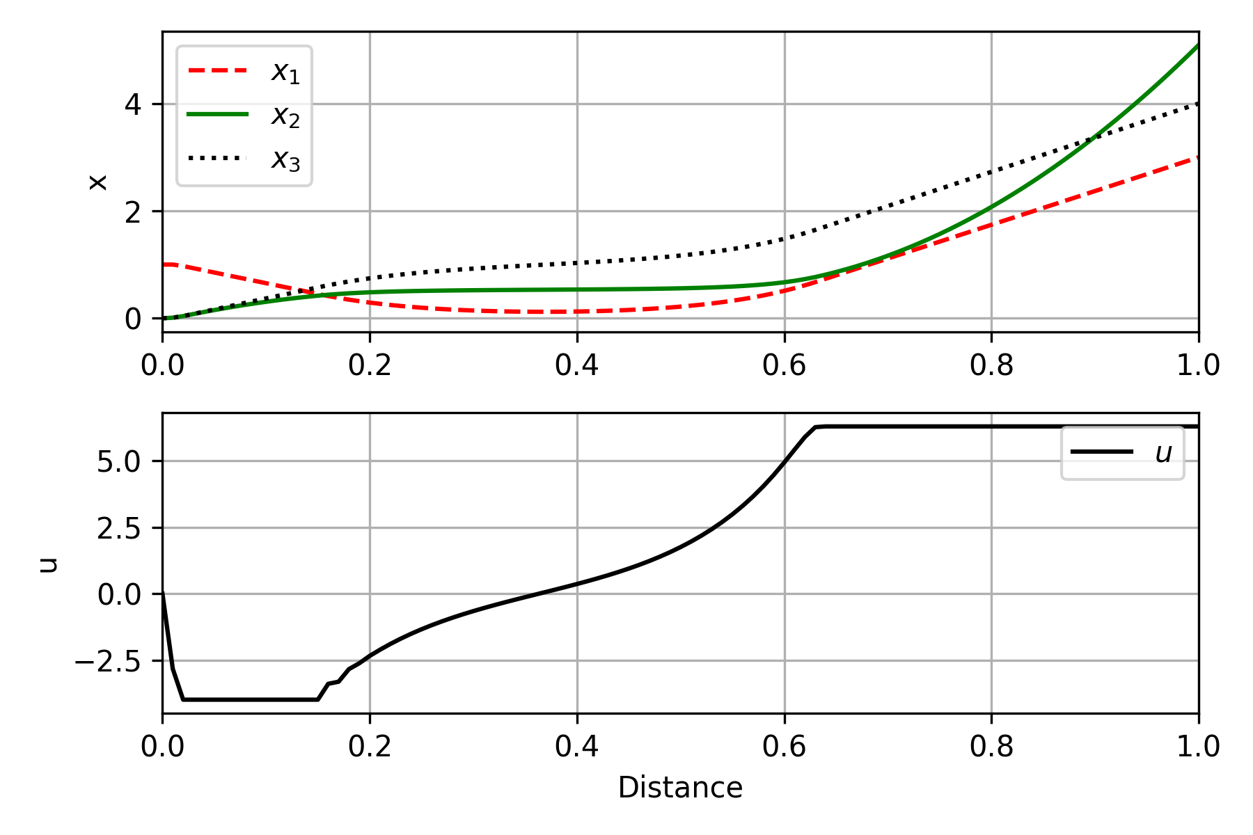
The objective of the hanging chain problem is to find the position of a chain of uniform density and length suspended between two points `a` and `b`. The problem is solved by minimizing the potential energy. This problem is from the COPS benchmark set. The equations are
$$ \begin{array}{llcl} \min_{x, u} & x_2(t_f) \\ \mbox{s.t.} & \dot{x}_1 & = & u \\ & \dot{x}_2 & = & x_1 (1+u^2)^{1/2} \\ & \dot{x}_3 & = & (1+u^2)^{1/2} \\ & x(t_0) &=& (a,0,0)^T \\ & x_1(t_f) &=& b \\ & x_3(t_f) &=& Lp \\ & x(t) &\in& [0,10] \\ & u(t) &\in& [-10,20] \end{array} $$
The parameters of this model are defined as `a=1`, `b=3`, and `Lp=4` with `t` from 0 to 1.

import numpy as np
import matplotlib.pyplot as plt
m = GEKKO(remote=False)
n = 101; Lp = 4; b = 3; a = 1
m.time = np.linspace(0,1,n)
x1,x2,x3 = m.Array(m.Var,3,lb=0,ub=10)
x1.value = a
u = m.MV(value=0, lb=-10, ub=20) # integer=True
z = np.zeros(n); z[-1] = 1
final = m.Param(value=z)
m.Equation(x1.dt() == u)
m.Equation(x2.dt() == x1 * (1+u**2)**0.5)
m.Equation(x3.dt() == (1+u**2)**0.5)
m.Minimize(1000*(x1-b)**2*final)
m.Minimize(1000*(x3-Lp)**2*final)
m.options.SOLVER = 3
m.options.NODES = 3
m.options.IMODE = 6
m.Minimize(x2*final)
# initialize
u.STATUS = 0
m.solve()
# optimize
m.options.TIME_SHIFT = 0
u.STATUS = 1; u.DCOST = 1e-3
m.solve()
plt.figure(figsize=(6,4))
plt.subplot(2,1,1)
plt.plot(m.time,x1.value,'r--',label=r'$x_1$')
plt.plot(m.time,x2.value,'g-',label=r'$x_2$')
plt.plot(m.time,x3.value,'k:',label=r'$x_3$')
plt.ylabel('x'); plt.xlim([0,1])
plt.legend(); plt.grid()
plt.subplot(2,1,2)
plt.plot(2,1,2)
plt.plot(m.time,u.value,'k-',label=r'$u$')
plt.grid(); plt.xlim([0,1]); plt.legend()
plt.xlabel('Distance'); plt.ylabel('u')
plt.tight_layout()
plt.savefig('chain.png',dpi=300); plt.show()


The Gekko Optimization Suite is a machine learning and optimization package in Python for mixed-integer and differential algebraic equations.
📄 Gekko Publication and References
The GEKKO package is available in Python with pip install gekko. There are additional example problems for equation solving, optimization, regression, dynamic simulation, model predictive control, and machine learning.