Dynamic Estimation Tuning
Dynamic estimation tuning is the process of adjusting certain objective function terms to give more desirable solutions. As an example, a dynamic estimation application such as moving horizon estimation (MHE) may either track noisy data too closely or the updates may be too slow to catch unmeasured disturbances of interest. Tuning is the process of achieving acceptable estimator performance based on unique aspects of the application.
Common Tuning Parameters for MHE
Tuning typically involves adjustment of objective function terms or constraints that limit the rate of change (DMAX), penalize the rate of change (DCOST), or set absolute bounds (LOWER and UPPER). Measurement availability is indicated by the parameter (FSTATUS). The optimizer can also include (1=on) or exclude (0=off) a certain adjustable parameter (FV) or manipulated variable (MV) with STATUS. Another important tuning consideration is the time horizon length. Including more points in the time horizon allows the estimator to reconcile the model to more data but also increases computational time.
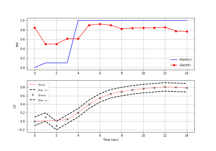

Below are common application, FV, MV, and CV tuning constants that are adjusted to achieve desired model predictive control performance.
- Application tuning
- DIAGLEVEL = diagnostic level (0-10) for solution information
- EV_TYPE = 1 for l1-norm and 2 for squared error objective
- IMODE = 5 or 8 for moving horizon estimation
- MAX_ITER = maximum iterations
- MAX_TIME = maximum time before stopping
- MV_TYPE = Set default MV type with 0=zero-order hold, 1=linear interpolation
- SOLVER
- 0=Try all available solvers
- 1=APOPT (MINLP, Active Set SQP)
- 2=BPOPT (NLP, Interior Point, SQP)
- 3=IPOPT (NLP, Interior Point, SQP)
- Fixed Value (FV) - single parameter value over time horizon
- DMAX = maximum that FV can move each cycle
- LOWER = lower FV bound
- FSTATUS = feedback status with 1=measured, 0=off
- STATUS = turn on (1) or off (0) FV
- UPPER = upper FV bound
- Manipulated Variable (MV) - parameter can change over time horizon
- COST = (+) minimize MV, (-) maximize MV
- DCOST = penalty for MV movement
- DMAX = maximum that MV can move each cycle
- FSTATUS = feedback status with 1=measured, 0=off
- LOWER = lower MV bound
- MV_TYPE = MV type with 0=zero-order hold, 1=linear interpolation
- STATUS = turn on (1) or off (0) MV
- UPPER = upper MV bound
- Controlled Variable (CV) tuning
- COST = (+) minimize MV, (-) maximize MV
- FSTATUS = feedback status with 1=measured, 0=off
- MEAS_GAP = measurement gap for estimator dead-band
There are several ways to change the tuning values. Tuning values can either be specified before an application is initialized or while an application is running. To change a tuning value before the application is loaded, use the apm_option() function such as the following example to change the lower bound in MATLAB or Python for the FV named p.
apm_option(server,app,'p.LOWER',0)
The upper and lower measurement deadband for a CV named y are set to values around the measurement. In this case, an acceptable range for the model prediction is to intersect the measurement of 10.0 between 9.5 and 10.5 with a MEAS_GAP of 1.0 (or +/-0.5).
apm_option(server,app,'y.MEAS_GAP',1.0)
Application constants are modified by indicating that the constant belongs to the group apm. IMODE is adjusted to either solve the MHE problem with a simultaneous (5) or sequential (8) method. In the case below, the application IMODE is changed to simultaneous mode.
apm_option(server,app,'apm.IMODE',5)
Exercise
Objective: Design an estimator to predict an unknown parameters so that a simple model is able to predict the response of a more complex process. Tune the estimator to achieve either tracking or predictive performance. Estimated time: 1 hour.
from random import random
from gekko import GEKKO
import matplotlib.pyplot as plt
n = 1 # process model order
#%% Process
rmt = False
p = GEKKO(remote=rmt)
p.time = [0,.5]
#Parameters
p.u = p.MV(value=0)
p.K = p.Param(value=1) #gain
p.tau = p.Param(value=5) #time constant
#Intermediate
p.x = [p.Intermediate(p.u)]
#Variables
p.x.extend([p.Var() for _ in range(n)]) #state variables
p.y = p.SV() #measurement
#Equations
p.Equations([p.tau/n * p.x[i+1].dt() == -p.x[i+1] + p.x[i] for i in range(n)])
p.Equation(p.y == p.K * p.x[n])
#options
p.options.IMODE = 4
#%% Model
m = GEKKO(remote=rmt)
#0-20 by 0.5 -- discretization must match simulation
m.time = np.linspace(0,20,41)
#Parameters
m.u = m.MV() #input
m.K = m.FV(value=1, lb=0.3, ub=3) #gain
m.tau = m.FV(value=5, lb=1, ub=10) #time constant
#Variables
m.x = m.SV() #state variable
m.y = m.CV() #measurement
#Equations
m.Equations([m.tau * m.x.dt() == -m.x + m.u,
m.y == m.K * m.x])
#Options
m.options.IMODE = 5 #MHE
m.options.EV_TYPE = 1
# STATUS = 0, optimizer doesn't adjust value
# STATUS = 1, optimizer can adjust
m.u.STATUS = 0
m.K.STATUS = 1
m.tau.STATUS = 1
# FSTATUS = 0, no measurement
# FSTATUS = 1, measurement used to update model
m.u.FSTATUS = 1
m.K.FSTATUS = 0
m.tau.FSTATUS = 0
m.y.FSTATUS = 1
# DMAX = maximum movement each cycle
m.K.DMAX = 1
m.tau.DMAX = .1
# MEAS_GAP = dead-band for measurement / model mismatch
m.y.MEAS_GAP = 0.0
#%% problem configuration
# number of cycles
cycles = 50
# time vector
tm = np.linspace(0,25,51)
# noise level
noise = 0.25
# values of u change randomly over time every 10th step
u_meas = np.zeros(cycles)
step_u = 0
for i in range(0,cycles):
if ((i-1)%10) == 0:
# random step (-5 to 5)
step_u = step_u + (random()-0.5)*10
u_meas[i] = step_u
#%% run process and estimator for cycles
y_meas = np.zeros(cycles)
y_est = np.zeros(cycles)
k_est = np.zeros(cycles)*np.nan
tau_est = np.zeros(cycles)*np.nan
for i in range(cycles-1):
# process simulator
p.u.MEAS = u_meas[i]
p.solve()
r = (random()-0.5)*noise
y_meas[i] = p.y.value[1] + r # add noise
# estimator
m.u.MEAS = u_meas[i]
m.y.MEAS = y_meas[i]
m.solve()
y_est[i] = m.y.MODEL
k_est[i] = m.K.NEWVAL
tau_est[i] = m.tau.NEWVAL
plt.clf()
plt.subplot(4,1,1)
plt.plot(tm[0:i+1],y_meas[0:i+1],'b-')
plt.plot(tm[0:i+1],y_est[0:i+1],'r--')
plt.legend(('meas','pred'))
plt.ylabel('y')
plt.subplot(4,1,2)
plt.plot(tm[0:i+1],np.ones(i+1)*p.K.value[0],'b-')
plt.plot(tm[0:i+1],k_est[0:i+1],'r--')
plt.legend(('actual','pred'))
plt.ylabel('k')
plt.subplot(4,1,3)
plt.plot(tm[0:i+1],np.ones(i+1)*p.tau.value[0],'b-')
plt.plot(tm[0:i+1],tau_est[0:i+1],'r--')
plt.legend(('actual','pred'))
plt.ylabel('tau')
plt.subplot(4,1,4)
plt.plot(tm[0:i+1],u_meas[0:i+1],'b-')
plt.legend('u')
plt.draw()
plt.pause(0.05)
Design an estimator to predict K and tau of a 1st order model to predict the dynamic response of a 1st order, 2nd order, and 10th order process. For the 2nd and 10th order systems, there is process/model mismatch. This means that the structure of the model can never exactly match the actual process because the equations are inherently incorrect. The parameter values are adjusted to best approximate the process even though the model is deficient. The process order is adjusted in the file process.apm file in the Constants section.
 Constants
   ! process model order
   n = 1  ! change to 1, 2, and 10
In each case, tune the estimator to favor either acceptable tracking or predictive performance. Tracking performance is the ability of the estimator to synchronize with measurements and is demonstrated with overall agreement between the model predictions and the measurements. Predictive performance sacrifices tracking performance to achieve more consistent values that are valid over a longer predictive horizon for model predictive control.
Solution
Jupyter Notebook Tip
For Jupyter notebooks, add the following code to allow real-time plots to display instead of creating a new plot for every frame. Use the clear_output() function in the loop where the plot is displayed.
display.clear_output(wait=True)
Here is a complete example:
import matplotlib.pyplot as plt
from IPython import display
x = np.linspace(0, 6 * np.pi, 100)
cos_values = []
sin_values = []
for i in range(len(x)):
# add the sin and cos of x at index i to the lists
cos_values.append(np.cos(x[i]))
sin_values.append(np.sin(x[i]))
# graph up until index i
plt.plot(x[:i], cos_values[:i], label='Cos')
plt.plot(x[:i], sin_values[:i], label='Sin')
plt.xlabel('input')
plt.ylabel('output')
# lines that help with animation
display.clear_output(wait=True) # replace figure
plt.pause(.01) # wait between figures
Discussion Questions
- If the measurements were noise-free and the model structure were perfect, which tuning parameters (DCOST, DMAX, MEAS_GAP, FSTATUS) would become unnecessary, and which would still matter? Why?
- What does a large MEAS_GAP (measurement deadband) do to the estimated parameters when the process drifts slowly? When is ignoring small mismatches exactly what you want, and when does it mask a developing fault?
- Your estimator uses a first-order model but the true process is 10th order. The estimator still "fits" - what do the estimated K and tau now mean, and why do they change with the input excitation used?
- The estimation horizon is a window into the past. What information is lost when the window slides forward, and what role does the prior (arrival-cost-like) penalty on parameter changes play in retaining it?
Generative AI Learning
Use these prompts after completing the estimator design exercise. Direct the AI - the tuning judgment is yours.
What to Turn In
Submit a short report (PDF, 1-2 pages) that curates your results into a demonstration of what you learned. You may use Generative AI to help write the report, but you must guide it to the correct visualizations, justifications, and assumptions. Answer these questions:
- Show your estimator tracking K and tau against the 1st, 2nd, and 10th-order processes (plots), with your final tuning values in a table.
- Present two tunings of the same estimator: one tuned for tracking, one for predictive performance. What did you change and what is the observable difference?
- For the 10th-order process: what do your estimated K and tau actually represent, and why is that still useful (or not) for control?
- From the committee prompt: the sharpest question you were asked and your corrected answer.