Dynamic control is also known as Nonlinear Model Predictive Control (NMPC) or simply as Nonlinear Control (NLC). NLC with predictive models is a dynamic optimization approach that seeks to follow a trajectory or drive certain values to maximum or minimum levels.

Exercise

Objective: Design a controller to maintain temperature of a chemical reactor. Develop 3 separate controllers (PID, Linear MPC, Nonlinear MPC) in Python, MATLAB, or Simulink. Demonstrate controller performance with steps in the set point and disturbance changes. Estimated time: 3 hours.

CSTR Source Files | Problem Information

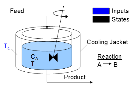
A reactor is used to convert a hazardous chemical A to an acceptable chemical B in waste stream before entering a nearby lake. This particular reactor is dynamically modeled as a Continuously Stirred Tank Reactor (CSTR) with a simplified kinetic mechanism that describes the conversion of reactant A to product B with an irreversible and exothermic reaction. It is desired to maintain the temperature at a constant setpoint that maximizes the destruction of A (highest possible temperature). Adjust the jacket temperature (T_c) to maintain a desired reactor temperature and minimize the concentration of A. The reactor temperature should never exceed 400 K. The cooling jacket temperature can be adjusted between 250 K and 350 K.

Step Testing

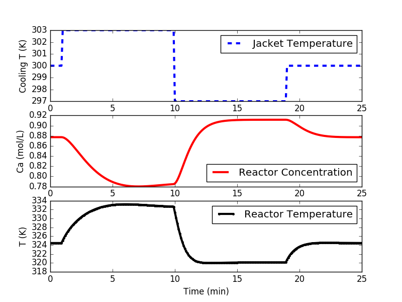
Step testing is required to obtain a process model for the PID controller and the linear model predictive controller. It is a first step in developing a controller. The following code implements either a doublet test or multiple steps to different levels. A doublet test starts with the system at steady state. Three moves of Manipulated Variable (MV) are made with sufficient time to nearly reach steady state conditions at two other operating points. The steps are above and below the nominal operating conditions. In this case, the cooling jacket temperature is raised, lowered, and brought back to 300 K (nominal operating condition.

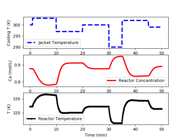
Additional steps are preferred for systems that show a high degree a nonlinearity or when there is little additional expense to obtain the data. The following code generates data at multiple input levels and with varying different step time intervals. The cooling jacket temperature is not raised above 305 K to avoid reactor instability in open loop.

Model Identification

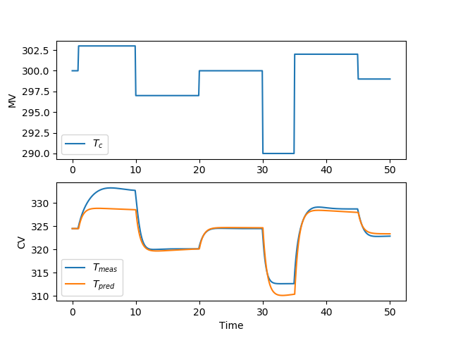
There are many methods to develop a controller model. For a PID controller, an FOPDT model is one method to obtain IMC tuning parameters. For linear MPC, there are many options to obtain a controller model through identification methods. For nonlinear MPC, the nonlinear simulator equations can be used to develop the controller. This section demonstrates how to obtain a linear model for the MPC application using the step test data generated in the prior section.

from gekko import GEKKO
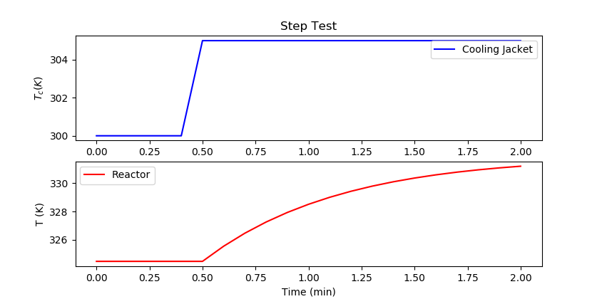
import pandas as pd
import matplotlib.pyplot as plt
import numpy as np

# load data and parse into columns
url = 'http://apmonitor.com/do/uploads/Main/cstr_step_tests.txt'
data = pd.read_csv(url)
print(data.head())

# generate time-series model
t = data['Time']
u = data['Tc']
y = data['T']
m = GEKKO(remote=True)

# system identification
na = 2 # output coefficients
nb = 2 # input coefficients
yp,p,K = m.sysid(t,u,y,na,nb,shift='init',scale=True,objf=100,diaglevel=1)

# plot results of fitting
plt.figure()
plt.subplot(2,1,1)
plt.plot(t,u)
plt.legend([r'$T_c$'])
plt.ylabel('MV')
plt.subplot(2,1,2)
plt.plot(t,y)
plt.plot(t,yp)
plt.legend([r'$T_{meas}$',r'$T_{pred}$'])
plt.ylabel('CV')
plt.xlabel('Time')
plt.savefig('sysid.png')

# step test model
yc,uc = m.arx(p)

# rename MV and CV
Tc = uc[0]
T = yc[0]

# steady state initialization
m.options.IMODE = 1
Tc.value = 300
m.solve(disp=False)

# dynamic simulation (step test validation)
m.time = np.linspace(0,2,21)
m.options.IMODE = 4
Tc.value = np.ones(21)*300
Tc.value[5:] = 305
m.solve(disp=False)

plt.figure()
plt.subplot(2,1,1)
plt.title('Step Test')
plt.plot(m.time,Tc.value,'b-',label='Cooling Jacket')
plt.ylabel(r'$T_c (K)$')
plt.legend()
plt.subplot(2,1,2)
plt.plot(m.time,T.value,'r-',label='Reactor')
plt.ylabel('T (K)')
plt.xlabel('Time (min)')
plt.legend()

plt.show()

[$[Get Code]]

Predictive Control

Linear MPC: Reactor Runaway and Upper Limit Temperature Violation (>400K)

import numpy as np
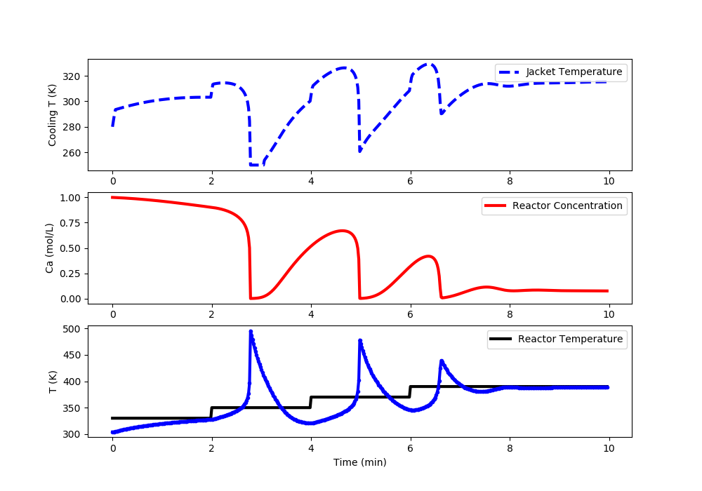
import matplotlib.pyplot as plt
from scipy.integrate import odeint
from gekko import GEKKO

# Steady State Initial Condition
u_ss = 280.0
# Feed Temperature (K)
Tf = 350
# Feed Concentration (mol/m^3)
Caf = 1

# Steady State Initial Conditions for the States
Ca_ss = 1
T_ss = 304
x0 = np.empty(2)
x0[0] = Ca_ss
x0[1] = T_ss

#%% GEKKO linear MPC
m = GEKKO(remote=True)
m.time = [0,0.02,0.04,0.06,0.08,0.1,0.15,0.2,0.3,0.4,0.5]

# initial conditions
Tc0 = 280
T0 = 304
Ca0 = 1.0

tau = m.Const(value = 0.5)
Kp = m.Const(value = 1)

m.Tc = m.MV(value = Tc0,lb=250,ub=350)
m.T = m.CV(value = T_ss)

m.Equation(tau * m.T.dt() == -(m.T - T0) + Kp * (m.Tc - Tc0))

#MV tuning
m.Tc.STATUS = 1
m.Tc.FSTATUS = 0
m.Tc.DMAX = 100
m.Tc.DMAXHI = 5   # constrain movement up
m.Tc.DMAXLO = -100 # quick action down
#CV tuning
m.T.STATUS = 1
m.T.FSTATUS = 1
m.T.SP = 330
m.T.TR_INIT = 2
m.T.TAU = 1.0
m.options.CV_TYPE = 2
m.options.IMODE = 6
m.options.SOLVER = 3

#%% define CSTR model
def cstr(x,t,u,Tf,Caf):
    # Inputs (3):
    # Temperature of cooling jacket (K)
    Tc = u
    # Tf = Feed Temperature (K)
    # Caf = Feed Concentration (mol/m^3)

    # States (2):
    # Concentration of A in CSTR (mol/m^3)
    Ca = x[0]
    # Temperature in CSTR (K)
    T = x[1]

    # Parameters:
    # Volumetric Flowrate (m^3/sec)
    q = 100
    # Volume of CSTR (m^3)
    V = 100
    # Density of A-B Mixture (kg/m^3)
    rho = 1000
    # Heat capacity of A-B Mixture (J/kg-K)
    Cp = 0.239
    # Heat of reaction for A->B (J/mol)
    mdelH = 5e4
    # E - Activation energy in the Arrhenius Equation (J/mol)
    # R - Universal Gas Constant = 8.31451 J/mol-K
    EoverR = 8750
    # Pre-exponential factor (1/sec)
    k0 = 7.2e10
    # U - Overall Heat Transfer Coefficient (W/m^2-K)
    # A - Area - this value is specific for the U calculation (m^2)
    UA = 5e4
    # reaction rate
    rA = k0*np.exp(-EoverR/T)*Ca

    # Calculate concentration derivative
    dCadt = q/V*(Caf - Ca) - rA
    # Calculate temperature derivative
    dTdt = q/V*(Tf - T) \
            + mdelH/(rho*Cp)*rA \
            + UA/V/rho/Cp*(Tc-T)

    # Return xdot:
    xdot = np.zeros(2)
    xdot[0] = dCadt
    xdot[1] = dTdt
    return xdot

# Time Interval (min)
t = np.linspace(0,10,501)

# Store results for plotting
Ca = np.ones(len(t)) * Ca_ss
T = np.ones(len(t)) * T_ss
Tsp = np.ones(len(t)) * T_ss
u = np.ones(len(t)) * u_ss

# Set point steps
Tsp[0:100] = 330.0
Tsp[100:200] = 350.0
Tsp[200:300] = 370.0
Tsp[300:] = 390.0

# Create plot
plt.figure(figsize=(10,7))
plt.ion()
plt.show()

# Simulate CSTR
for i in range(len(t)-1):
    # simulate one time period (0.05 sec each loop)
    ts = [t[i],t[i+1]]
    y = odeint(cstr,x0,ts,args=(u[i],Tf,Caf))
    # retrieve measurements
    Ca[i+1] = y[-1][0]
    T[i+1] = y[-1][1]
    # insert measurement
    m.T.MEAS = T[i+1]
    # update setpoint
    m.T.SP = Tsp[i+1]
    # solve MPC
    m.solve(disp=True)
    # change to a fixed starting point for trajectory
    m.T.TR_INIT = 2
    # retrieve new Tc value
    u[i+1] = m.Tc.NEWVAL
    # update initial conditions
    x0[0] = Ca[i+1]
    x0[1] = T[i+1]

    #%% Plot the results
    plt.clf()
    plt.subplot(3,1,1)
    plt.plot(t[0:i],u[0:i],'b--',lw=3)
    plt.ylabel('Cooling T (K)')
    plt.legend(['Jacket Temperature'],loc='best')

    plt.subplot(3,1,2)
    plt.plot(t[0:i],Ca[0:i],'r-',lw=3)
    plt.ylabel('Ca (mol/L)')
    plt.legend(['Reactor Concentration'],loc='best')

    plt.subplot(3,1,3)
    plt.plot(t[0:i],Tsp[0:i],'k-',lw=3,label=r'$T_{sp}$')
    plt.plot(t[0:i],T[0:i],'b.-',lw=3,label=r'$T_{meas}$')
    plt.ylabel('T (K)')
    plt.xlabel('Time (min)')
    plt.legend(['Reactor Temperature'],loc='best')
    plt.draw()
    plt.pause(0.01)

[$[Get Code]]

Linear ARX MPC: Reactor Runaway and Upper Limit Temperature Violation (>400K)

import numpy as np
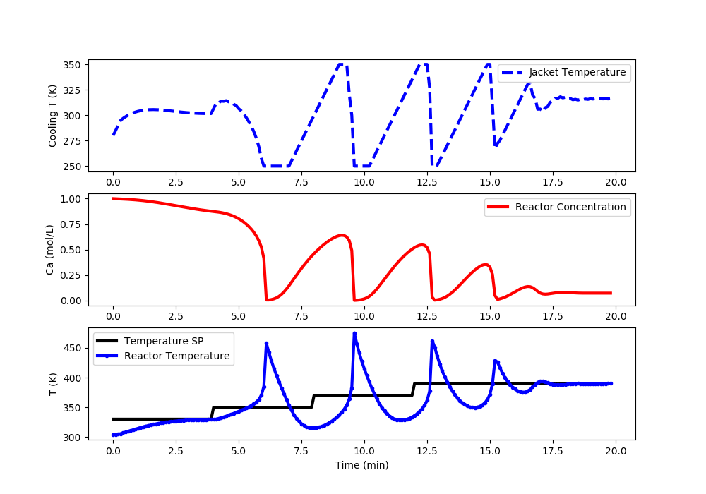
import matplotlib.pyplot as plt
from scipy.integrate import odeint
import pandas as pd
from gekko import GEKKO

# load data and parse into columns
url = 'http://apmonitor.com/do/uploads/Main/cstr_step_tests.txt'
data = pd.read_csv(url)
print(data.head())

# generate time-series model
t = data['Time']
u = data['Tc']
y = data['T']
m = GEKKO(remote=True)

# system identification
na = 2 # output coefficients
nb = 2 # input coefficients
yp,p,K = m.sysid(t,u,y,na,nb,shift='init',scale=True,objf=100,diaglevel=1)

# plot results of fitting
plt.figure()
plt.subplot(2,1,1)
plt.plot(t,u)
plt.legend([r'$T_c$'])
plt.ylabel('MV')
plt.subplot(2,1,2)
plt.plot(t,y)
plt.plot(t,yp)
plt.legend([r'$T_{meas}$',r'$T_{pred}$'])
plt.ylabel('CV')
plt.xlabel('Time')
plt.savefig('sysid.png')
plt.show()

# step test model
yc,uc = m.arx(p)

# rename MV and CV
m.Tc = uc[0]
m.T = yc[0]

# steady state initialization
m.options.IMODE = 1
m.Tc.value = 280
m.solve(disp=True)

# GEKKO linear MPC
m.time = np.linspace(0,2,21)

# MV tuning
m.Tc.STATUS = 1
m.Tc.FSTATUS = 0
m.Tc.DMAX = 100
m.Tc.DCOST = 0.1
m.Tc.DMAXHI = 5   # constrain movement up
m.Tc.DMAXLO = -100 # quick action down
m.Tc.UPPER = 350
m.Tc.LOWER = 250
# CV tuning
m.T.STATUS = 1
m.T.FSTATUS = 1
m.T.SP = 330
m.T.TR_INIT = 1
m.T.TAU = 1.2
m.options.CV_TYPE = 2
m.options.IMODE = 6
m.options.SOLVER = 3

# define CSTR (plant)
def cstr(x,t,Tc):
    Ca,T = x
    Tf = 350; Caf = 1.0; q = 100; V = 100
    rho = 1000; Cp = 0.239; mdelH = 5e4
    EoverR = 8750; k0 = 7.2e10; UA = 5e4
    rA = k0*np.exp(-EoverR/T)*Ca
    dCadt = q/V*(Caf - Ca) - rA
    dTdt = q/V*(Tf - T) + mdelH/(rho*Cp)*rA + UA/V/rho/Cp*(Tc-T)
    return [dCadt,dTdt]

# Time Interval (min)
t = np.linspace(0,20,201)

# Store results for plotting
Ca_ss = 1; T_ss = 304; Tc_ss = 280
Ca = np.ones(len(t)) * Ca_ss
T = np.ones(len(t)) * T_ss
Tsp = np.ones(len(t)) * T_ss
Tc = np.ones(len(t)) * Tc_ss

# Set point steps
Tsp[0:40] = 330.0
Tsp[40:80] = 350.0
Tsp[80:120] = 370.0
Tsp[120:] = 390.0

# Create plot
plt.figure(figsize=(10,7))
plt.ion()
plt.show()

# Simulate CSTR
x0 = [Ca_ss,T_ss]
for i in range(len(t)-1):
    y = odeint(cstr,x0,[0,0.05],args=(Tc[i],))
    # retrieve measurements
    Ca[i+1] = y[-1][0]
    T[i+1] = y[-1][1]
    # insert measurement
    m.T.MEAS = T[i+1]
    # update setpoint
    m.T.SP = Tsp[i+1]
    # solve MPC
    m.solve(disp=True)
    # retrieve new Tc value
    Tc[i+1] = m.Tc.NEWVAL
    # update initial conditions
    x0[0] = Ca[i+1]
    x0[1] = T[i+1]

    #%% Plot the results
    plt.clf()
    plt.subplot(3,1,1)
    plt.plot(t[0:i],Tc[0:i],'b--',lw=3)
    plt.ylabel('Cooling T (K)')
    plt.legend(['Jacket Temperature'],loc='best')

    plt.subplot(3,1,2)
    plt.plot(t[0:i],Ca[0:i],'r-',lw=3)
    plt.ylabel('Ca (mol/L)')
    plt.legend(['Reactor Concentration'],loc='best')

    plt.subplot(3,1,3)
    plt.plot(t[0:i],Tsp[0:i],'k-',lw=3,label=r'$T_{sp}$')
    plt.plot(t[0:i],T[0:i],'b.-',lw=3,label=r'$T_{meas}$')
    plt.ylabel('T (K)')
    plt.xlabel('Time (min)')
    plt.legend(['Temperature SP','Reactor Temperature'],loc='best')
    plt.draw()
    plt.pause(0.01)

[$[Get Code]]

Nonlinear MPC: Acceptable Temperature (<400K) and Concentration (<0.2) Control

import numpy as np
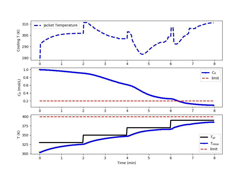
import matplotlib.pyplot as plt
from scipy.integrate import odeint
from gekko import GEKKO

# Steady State Initial Condition
u_ss = 280.0
# Feed Temperature (K)
Tf = 350
# Feed Concentration (mol/m^3)
Caf = 1

# Steady State Initial Conditions for the States
Ca_ss = 1
T_ss = 304
x0 = np.empty(2)
x0[0] = Ca_ss
x0[1] = T_ss

#%% GEKKO nonlinear MPC
m = GEKKO(remote=True)
m.time = [0,0.02,0.04,0.06,0.08,0.1,0.12,0.15,0.2]

# Volumetric Flowrate (m^3/sec)
q = 100
# Volume of CSTR (m^3)
V = 100
# Density of A-B Mixture (kg/m^3)
rho = 1000
# Heat capacity of A-B Mixture (J/kg-K)
Cp = 0.239
# Heat of reaction for A->B (J/mol)
mdelH = 5e4
# E - Activation energy in the Arrhenius Equation (J/mol)
# R - Universal Gas Constant = 8.31451 J/mol-K
EoverR = 8750
# Pre-exponential factor (1/sec)
k0 = 7.2e10
# U - Overall Heat Transfer Coefficient (W/m^2-K)
# A - Area - this value is specific for the U calculation (m^2)
UA = 5e4

# initial conditions
Tc0 = 280
T0 = 304
Ca0 = 1.0

tau = m.Const(value=0.5)
Kp = m.Const(value=1)

m.Tc = m.MV(value=Tc0,lb=250,ub=350)
m.T = m.CV(value=T_ss)
m.rA = m.Var(value=0)
m.Ca = m.CV(value=Ca_ss)

m.Equation(m.rA == k0*m.exp(-EoverR/m.T)*m.Ca)

m.Equation(m.T.dt() == q/V*(Tf - m.T) \
            + mdelH/(rho*Cp)*m.rA \
            + UA/V/rho/Cp*(m.Tc-m.T))

m.Equation(m.Ca.dt() == q/V*(Caf - m.Ca) - m.rA)

#MV tuning
m.Tc.STATUS = 1
m.Tc.FSTATUS = 0
m.Tc.DMAX = 100
m.Tc.DMAXHI = 20   # constrain movement up
m.Tc.DMAXLO = -100 # quick action down

#CV tuning
m.T.STATUS = 1
m.T.FSTATUS = 1
m.T.TR_INIT = 1
m.T.TAU = 1.0
DT = 0.5 # deadband

m.Ca.STATUS = 0
m.Ca.FSTATUS = 0 # no measurement
m.Ca.TR_INIT = 0

m.options.CV_TYPE = 1
m.options.IMODE = 6
m.options.SOLVER = 3

#%% define CSTR model
def cstr(x,t,u,Tf,Caf):
    # Inputs (3):
    # Temperature of cooling jacket (K)
    Tc = u
    # Tf = Feed Temperature (K)
    # Caf = Feed Concentration (mol/m^3)

    # States (2):
    # Concentration of A in CSTR (mol/m^3)
    Ca = x[0]
    # Temperature in CSTR (K)
    T = x[1]

    # Parameters:
    # Volumetric Flowrate (m^3/sec)
    q = 100
    # Volume of CSTR (m^3)
    V = 100
    # Density of A-B Mixture (kg/m^3)
    rho = 1000
    # Heat capacity of A-B Mixture (J/kg-K)
    Cp = 0.239
    # Heat of reaction for A->B (J/mol)
    mdelH = 5e4
    # E - Activation energy in the Arrhenius Equation (J/mol)
    # R - Universal Gas Constant = 8.31451 J/mol-K
    EoverR = 8750
    # Pre-exponential factor (1/sec)
    k0 = 7.2e10
    # U - Overall Heat Transfer Coefficient (W/m^2-K)
    # A - Area - this value is specific for the U calculation (m^2)
    UA = 5e4
    # reaction rate
    rA = k0*np.exp(-EoverR/T)*Ca

    # Calculate concentration derivative
    dCadt = q/V*(Caf - Ca) - rA
    # Calculate temperature derivative
    dTdt = q/V*(Tf - T) \
            + mdelH/(rho*Cp)*rA \
            + UA/V/rho/Cp*(Tc-T)

    # Return xdot:
    xdot = np.zeros(2)
    xdot[0] = dCadt
    xdot[1] = dTdt
    return xdot

# Time Interval (min)
t = np.linspace(0,8,401)

# Store results for plotting
Ca = np.ones(len(t)) * Ca_ss
T = np.ones(len(t)) * T_ss
Tsp = np.ones(len(t)) * T_ss
u = np.ones(len(t)) * u_ss

# Set point steps
Tsp[0:100] = 330.0
Tsp[100:200] = 350.0
Tsp[200:300] = 370.0
Tsp[300:] = 390.0

# Create plot
plt.figure(figsize=(10,7))
plt.ion()
plt.show()

# Simulate CSTR
for i in range(len(t)-1):
    # simulate one time period (0.05 sec each loop)
    ts = [t[i],t[i+1]]
    y = odeint(cstr,x0,ts,args=(u[i],Tf,Caf))
    # retrieve measurements
    Ca[i+1] = y[-1][0]
    T[i+1] = y[-1][1]
    # insert measurement
    m.T.MEAS = T[i+1]
    # solve MPC
    m.solve(disp=True)

    m.T.SPHI = Tsp[i+1] + DT
    m.T.SPLO = Tsp[i+1] - DT

    # retrieve new Tc value
    u[i+1] = m.Tc.NEWVAL
    # update initial conditions
    x0[0] = Ca[i+1]
    x0[1] = T[i+1]

    #%% Plot the results
    plt.clf()
    plt.subplot(3,1,1)
    plt.plot(t[0:i],u[0:i],'b--',lw=3)
    plt.ylabel('Cooling T (K)')
    plt.legend(['Jacket Temperature'],loc='best')

    plt.subplot(3,1,2)
    plt.plot(t[0:i],Ca[0:i],'b.-',lw=3,label=r'$C_A$')
    plt.plot([0,t[i-1]],[0.2,0.2],'r--',lw=2,label='limit')
    plt.ylabel(r'$C_A$ (mol/L)')
    plt.legend(loc='best')

    plt.subplot(3,1,3)
    plt.plot(t[0:i],Tsp[0:i],'k-',lw=3,label=r'$T_{sp}$')
    plt.plot(t[0:i],T[0:i],'b.-',lw=3,label=r'$T_{meas}$')
    plt.plot([0,t[i-1]],[400,400],'r--',lw=2,label='limit')
    plt.ylabel('T (K)')
    plt.xlabel('Time (min)')
    plt.legend(loc='best')
    plt.draw()
    plt.pause(0.01)

[$[Get Code]]

See additional information on this application with CSTR PID Control with MATLAB and CSTR PID Control with Python.

Solution in Python

PID for CSTR Control (Python) - Solution Video

Linear MPC for CSTR Control (APM Python) - Solution Video

Nonlinear MPC for CSTR Control (APM Python) - Solution Video

Solution in Simulink

PID for CSTR Control (Simulink) - Solution Video

Linear MPC for CSTR Control (Simulink) - Solution Video

Nonlinear MPC for CSTR Control (Simulink) - Solution Video

Generative AI Learning

Use these prompts for the CSTR control exercises (PID, linear MPC, nonlinear MPC). The comparison and its explanation are the graded skill - the AI is your committee, not your co-author.

What to Turn In

Submit a short report (PDF, 1-2 pages) that curates your results into a demonstration of what you learned. You may use Generative AI to help write the report, but you must guide it to the correct visualizations, justifications, and assumptions. Answer these questions:

1. Include the setpoint-ladder plots (330 to 390 K) for PID, linear MPC, and nonlinear MPC, and a table comparing them (IAE or similar, worst overshoot vs the 400 K limit, MV effort, solve time per cycle).
2. Where exactly does the linear controller start to fail, and what property of the reactor at that operating point explains it?
3. How did you implement the 400 K limit (hard vs soft), and what failure scenario justifies your choice over the alternative?
4. From the debugging prompt (or your own solver failure): the symptom, your committed diagnosis, and the evidence that confirmed or refuted it.