Temperature Control of a Stirred Reactor
 |  |  |
|---|
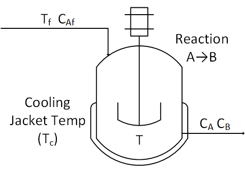
The objective of this case study is to automatically maintain a temperature in stirred tank reactor with a highly exothermic reaction. This is an example of a highly nonlinear process that is prone to exponential run-away when the temperature rises too quickly.
A reactor is used to convert a hazardous chemical A to an acceptable chemical B in waste stream before entering a nearby lake. This particular reactor is dynamically modeled as a Continuously Stirred Tank Reactor (CSTR) with a simplified kinetic mechanism that describes the conversion of reactant A to product B with an irreversible and exothermic reaction. Because the analyzer for product B is not fast enough for real-time control, it is desired to maintain the temperature at a constant set point that maximizes the consumption of A (highest possible temperature).
Run the Python app with streamlit. A browser window opens with the app interface.
streamlit run app_cstr_pid.py
The objectives of this exercise are to:
- Create a dynamic first-order model
- Obtain PID tuning parameters
- Adjusting the PID tuning or implement other strategies to achieve acceptable performance
- Final concentration target < 0.1 without temperature run-away (T<400K)

Doublet Test for FOPDT Fit
Perform the necessary open loop tests to determine a first order plus dead time (FOPDT) model that describes the relationship between cooling jacket temperature (MV=Tc) and reactor temperature (CV=T). Use the file data.txt to extract the information for the FOPDT model. Obtain an FOPDT model and report the values of the three parameters `K_p, \tau_p, \theta_p`.
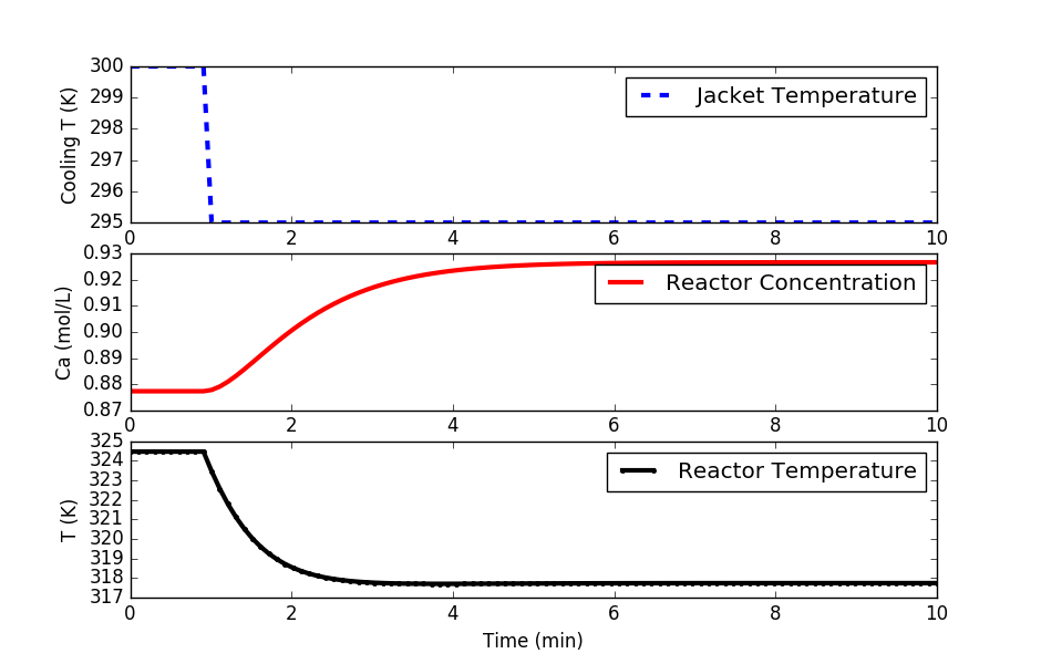
Below is a step test example in Python. Modify this to start at 300K for the cooling jacket temperature, step up to 303K, down to 297K, and back to 300K in a doublet test. Fit `K_p, \tau_p, \theta_p` of an FOPDT model using optimization to achieve the best match to the simulated CSTR data.
import matplotlib.pyplot as plt
from scipy.integrate import odeint
# animate plots?
animate=True # True / False
# define CSTR model
def cstr(x,t,u,Tf,Caf):
# Inputs (3):
# Temperature of cooling jacket (K)
Tc = u
# Tf = Feed Temperature (K)
# Caf = Feed Concentration (mol/m^3)
# States (2):
# Concentration of A in CSTR (mol/m^3)
Ca = x[0]
# Temperature in CSTR (K)
T = x[1]
# Parameters:
# Volumetric Flowrate (m^3/sec)
q = 100
# Volume of CSTR (m^3)
V = 100
# Density of A-B Mixture (kg/m^3)
rho = 1000
# Heat capacity of A-B Mixture (J/kg-K)
Cp = 0.239
# Heat of reaction for A->B (J/mol)
mdelH = 5e4
# E - Activation energy in the Arrhenius Equation (J/mol)
# R - Universal Gas Constant = 8.31451 J/mol-K
EoverR = 8750
# Pre-exponential factor (1/sec)
k0 = 7.2e10
# U - Overall Heat Transfer Coefficient (W/m^2-K)
# A - Area - this value is specific for the U calculation (m^2)
UA = 5e4
# reaction rate
rA = k0*np.exp(-EoverR/T)*Ca
# Calculate concentration derivative
dCadt = q/V*(Caf - Ca) - rA
# Calculate temperature derivative
dTdt = q/V*(Tf - T) \
+ mdelH/(rho*Cp)*rA \
+ UA/V/rho/Cp*(Tc-T)
# Return xdot:
xdot = np.zeros(2)
xdot[0] = dCadt
xdot[1] = dTdt
return xdot
# Steady State Initial Conditions for the States
Ca_ss = 0.87725294608097
T_ss = 324.475443431599
x0 = np.empty(2)
x0[0] = Ca_ss
x0[1] = T_ss
# Steady State Initial Condition
u_ss = 300.0
# Feed Temperature (K)
Tf = 350
# Feed Concentration (mol/m^3)
Caf = 1
# Time Interval (min)
t = np.linspace(0,10,100)
# Store results for plotting
Ca = np.ones(len(t)) * Ca_ss
T = np.ones(len(t)) * T_ss
u = np.ones(len(t)) * u_ss
# Step cooling temperature to 295
u[10:] = 295.0
plt.figure(1)
if animate:
plt.ion()
plt.show()
# Simulate CSTR
for i in range(len(t)-1):
ts = [t[i],t[i+1]]
y = odeint(cstr,x0,ts,args=(u[i+1],Tf,Caf))
Ca[i+1] = y[-1][0]
T[i+1] = y[-1][1]
x0[0] = Ca[i+1]
x0[1] = T[i+1]
# plot results
if animate:
plt.clf()
# Plot the results
plt.subplot(3,1,1)
plt.plot(t[0:i+1],u[0:i+1],'b--',linewidth=3)
plt.ylabel('Cooling T (K)')
plt.legend(['Jacket Temperature'],loc='best')
plt.subplot(3,1,2)
plt.plot(t[0:i+1],Ca[0:i+1],'r-',linewidth=3)
plt.ylabel('Ca (mol/L)')
plt.legend(['Reactor Concentration'],loc='best')
plt.subplot(3,1,3)
plt.plot(t[0:i+1],T[0:i+1],'k.-',linewidth=3)
plt.ylabel('T (K)')
plt.xlabel('Time (min)')
plt.legend(['Reactor Temperature'],loc='best')
plt.pause(0.01)
# Construct results and save data file
# Column 1 = time
# Column 2 = cooling temperature
# Column 3 = reactor temperature
data = np.vstack((t,u,T)) # vertical stack
data = data.T # transpose data
np.savetxt('data.txt',data,delimiter=',')
# Plot the results
if not animate:
plt.subplot(3,1,1)
plt.plot(t,u,'b--',linewidth=3)
plt.ylabel('Cooling T (K)')
plt.legend(['Jacket Temperature'],loc='best')
plt.subplot(3,1,2)
plt.plot(t,Ca,'r-',linewidth=3)
plt.ylabel('Ca (mol/L)')
plt.legend(['Reactor Concentration'],loc='best')
plt.subplot(3,1,3)
plt.plot(t,T,'k.-',linewidth=3)
plt.ylabel('T (K)')
plt.xlabel('Time (min)')
plt.legend(['Reactor Temperature'],loc='best')
plt.show()
Design PI or PID Controller
Use the `K_p, \tau_p, \theta_p` from the FOPDT model in the Internal Model Control (IMC) PI tuning correlation or PID tuning correlation to obtain starting values of `K_c`, `\tau_I`, and `\tau_D` for a PI or PID controller. Use an aggressive value for the closed loop time constant, `\tau_c = 0.1 \tau_p`.
Implement PI or PID Controller
Using `K_c`, `\tau_I`, and `\tau_D` from the IMC tuning correlation, implement a PID controller with anti-reset windup. Test the set point tracking capability of this controller by plotting the response of the process to steps in set point of the reactor temperature (not cooling jacket temperature) from 300K up to 320K and then down to 280K. Limit the cooling jacket temperature between 250K and 350K. Comment on how the nonlinear behavior of this process impacts your observed set point response performance.
Tune PI or PID Controller
Improve the tuning by adjusting `K_c`, `\tau_I`, and `\tau_D` by trial and error until the controller displays a 10% to 15% overshoot in response to a reactor temperature set point step from 300K to 320K. Plot this set point step response.
Challenge: Lowest Concentration
Step up the set point to achieve a maximum temperature in the reactor without exceeding the maximum allowable temperature of 400K (don’t cause a reactor run-away). What is the lowest concentration that can be achieved without exceeding the maximum allowable temperature? This is a very difficult problem due to the potential for reactor temperature run-away. Derivative action may be necessary to achieve the best performance.
The following code is an implementation of a PID controller but is unable to keep the reactor temperature below the upper limit of 400K.
import matplotlib.pyplot as plt
from scipy.integrate import odeint
from simple_pid import PID # pip install simple_pid
import time
make_gif = True
try:
import imageio # required to make gif animation
except:
print('install imageio with "pip install imageio" to make gif')
make_gif=False
if make_gif:
try:
import os
images = []
os.mkdir('./frames')
except:
pass
# define CSTR model
def cstr(x,t,u,Tf,Caf):
# Inputs (3):
# Temperature of cooling jacket (K)
Tc = u
# Tf = Feed Temperature (K)
# Caf = Feed Concentration (mol/m^3)
# States (2):
# Concentration of A in CSTR (mol/m^3)
Ca = x[0]
# Temperature in CSTR (K)
T = x[1]
# Parameters:
# Volumetric Flowrate (m^3/sec)
q = 100
# Volume of CSTR (m^3)
V = 100
# Density of A-B Mixture (kg/m^3)
rho = 1000
# Heat capacity of A-B Mixture (J/kg-K)
Cp = 0.239
# Heat of reaction for A->B (J/mol)
mdelH = 5e4
# E - Activation energy in the Arrhenius Equation (J/mol)
# R - Universal Gas Constant = 8.31451 J/mol-K
EoverR = 8750
# Pre-exponential factor (1/sec)
k0 = 7.2e10
# U - Overall Heat Transfer Coefficient (W/m^2-K)
# A - Area - this value is specific for the U calculation (m^2)
UA = 5e4
# reaction rate
rA = k0*np.exp(-EoverR/T)*Ca
# Calculate concentration derivative
dCadt = q/V*(Caf - Ca) - rA
# Calculate temperature derivative
dTdt = q/V*(Tf - T) \
+ mdelH/(rho*Cp)*rA \
+ UA/V/rho/Cp*(Tc-T)
# Return xdot:
xdot = np.zeros(2)
xdot[0] = dCadt
xdot[1] = dTdt
return xdot
# Steady State Initial Conditions for the States
Ca_ss = 0.87725294608097
T_ss = 324.475443431599
x0 = np.empty(2)
x0[0] = Ca_ss
x0[1] = T_ss
# Steady State Initial Condition
u_ss = 300.0
# Feed Temperature (K)
Tf = 350
# Feed Concentration (mol/m^3)
Caf = 1
# Time Interval (min)
t = np.linspace(0,10,101)
# Store results for plotting
Ca = np.ones(len(t)) * Ca_ss
T = np.ones(len(t)) * T_ss
u = np.ones(len(t)) * u_ss
# setpoint
sp = np.ones(101) * T_ss
sp[5:] = 340.0
u_bias = u_ss
# create PID controller
# op = op_bias + Kc * e + Ki * ei + Kd * ed
# with ei = error integral
# with ed = error derivative
Kc = 1.0 # Controller gain
Ki = 1.0 # Controller integral parameter
Kd = 0.0 # Controller derivative parameter
pid = PID(Kc,Ki,Kd)
# lower and upper controller output limits
oplo = 250.0
ophi = 350.0
pid.output_limits = (oplo-u_bias,ophi-u_bias)
# PID sample time
pid.sample_time = 0.1
plt.figure(1)
plt.ion()
plt.show()
# timing functions
tm = np.zeros(101)
sleep_max = 0.101
start_time = time.time()
prev_time = start_time
# Simulate CSTR
for i in range(len(t)-1):
# PID control
pid.setpoint=sp[i]
u[i+1] = pid(T[i]) + u_bias
ts = [t[i],t[i+1]]
y = odeint(cstr,x0,ts,args=(u[i+1],Tf,Caf))
Ca[i+1] = y[-1][0]
T[i+1] = y[-1][1]
x0[0] = Ca[i+1]
x0[1] = T[i+1]
# plot results
plt.clf()
# Plot the results
plt.subplot(3,1,1)
plt.plot(t[0:i+1],u[0:i+1],'b--',linewidth=3)
plt.ylabel('Cooling T (K)')
plt.legend(['Jacket Temperature'],loc='best')
plt.subplot(3,1,2)
plt.plot(t[0:i+1],Ca[0:i+1],'r-',linewidth=3)
plt.ylabel('Ca (mol/L)')
plt.legend(['Reactor Concentration'],loc='best')
plt.subplot(3,1,3)
plt.plot([t[0],t[i]],[400.0,400.0],'r-',linewidth=2)
plt.plot(t[0:i+1],T[0:i+1],'b.-',linewidth=3)
plt.plot(t[0:i+1],sp[0:i+1],'k:',linewidth=3)
plt.ylabel('T (K)')
plt.xlabel('Time (min)')
plt.legend(['Upper Limit','Reactor Temperature','Set Point'],loc='best')
plt.pause(0.001)
if make_gif:
filename='./frames/frame_'+str(1000+i)+'.png'
plt.savefig(filename)
images.append(imageio.imread(filename))
# Sleep time
sleep = sleep_max - (time.time() - prev_time)
if sleep>=0.001:
time.sleep(sleep-0.001)
else:
time.sleep(0.001)
# Record time and change in time
ct = time.time()
dt = ct - prev_time
prev_time = ct
tm[i+1] = ct - start_time
# Construct results and save data file
# Column 1 = time
# Column 2 = cooling temperature
# Column 3 = reactor temperature
data = np.vstack((t,u,T)) # vertical stack
data = data.T # transpose data
np.savetxt('data.txt',data,delimiter=',')
# create animated GIF
if make_gif:
imageio.mimsave('animate.gif', images)
#imageio.mimsave('animate.mp4', images) # requires ffmpeg