Oil Shale Pyrolysis
Oil shale pyrolysis involves heating oil shale in the absence of oxygen to produce oil, gas, and solid residues. Oil shale is a sedimentary rock containing organic matter that can be converted into liquid and gaseous hydrocarbons under high temperature and pressure. The organic matter in oil shale breaks down into various hydrocarbons, such as oil, gas, and waxes. The resulting products are then separated and processed to produce usable fuels and chemicals. The solid residues left over after the pyrolysis process can also be used as fuel or as raw materials for other processes.
Optimizing oil shale pyrolysis is important for several reasons. First, oil shale is an abundant resource, and the pyrolysis process unlocks the potential as a source of energy and chemicals. Secondly, oil shale pyrolysis is a complex process that requires control of the temperature, pressure, and reaction time to maximize the yield and quality of the products. It is possible to increase the efficiency and reduce the cost of producing oil and gas from oil shale through optimization. Oil shale pyrolysis process has significant environmental impacts by releasing large amounts of greenhouse gases. By optimizing the process, it is possible to minimize these emissions and reduce the environmental impact.
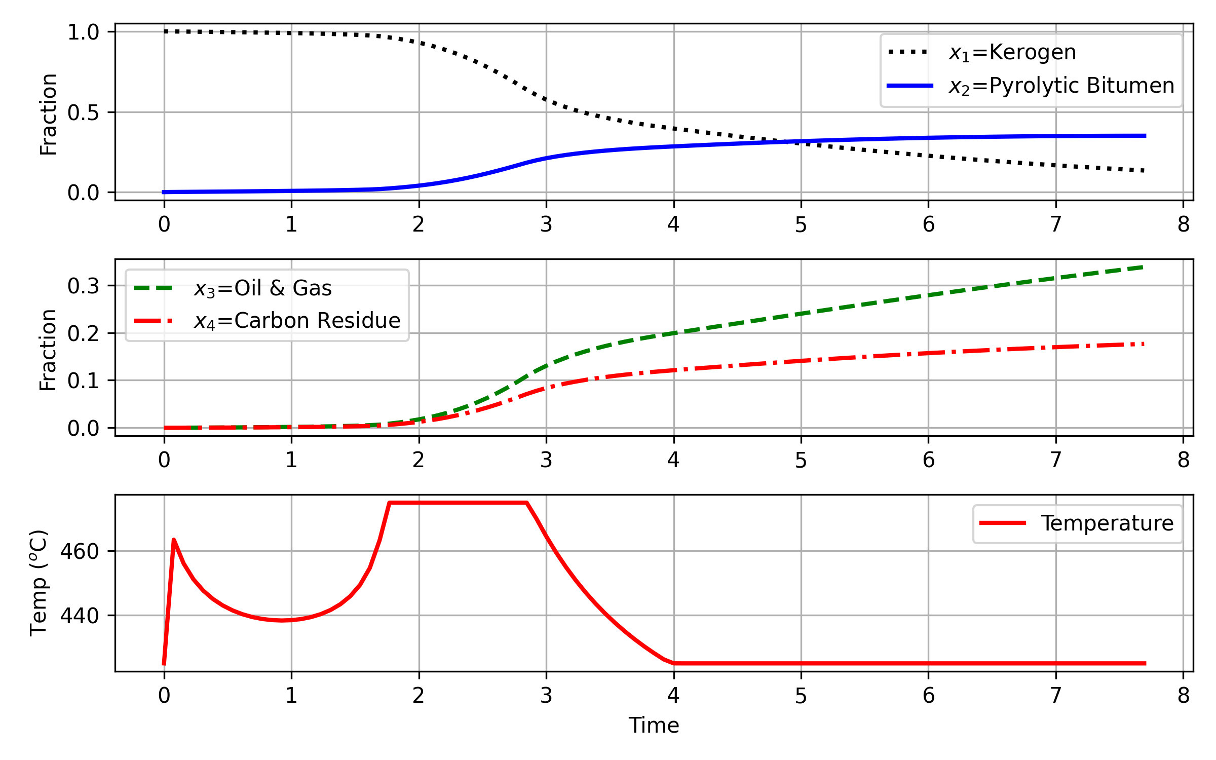
In a simplified model, oil shale pyrolysis starts with kerogen and is decomposed into pyrolytic bitumen, oil and gas, and residual carbon. The objective is to maximize the fraction of pyrolytic bitumen `x_2`. There are 5 reactions including:
$$A_1 \xrightarrow{k_1} A_2$$
$$A_2 \xrightarrow{k_2} A_3$$
$$A_1 + A_2 \xrightarrow{k_3} A_2 + A_2$$
$$A_1 + A_2 \xrightarrow{k_4} A_3 + A_2$$
$$A_1 + A_2 \xrightarrow{k_5} A_4 + A_2$$
Each reaction rate is:
$$k_i = k_{i0} \exp{\left(-E_i/RT\right)}, (i=1,2,3,4,5)$$
The optimization problem is:
$$ \begin{array}{lll} \max_{T} & &x_2(t_N) \\ \mbox{s.t.} & \dot{x}_1 &= -k_1x_1-(k_3+k_4+k_5)x_1x_2\\ & \dot{x}_2 &= k_1x_1-k_2x_2 + k_3x_1x_2\\ & \dot{x}_3 &= k_2x_2 + k_4x_1x_2\\ & \dot{x}_4 &= k_5x_1x_2\\ & k_i &= a_i e^{-\frac{b_i}{RT}},\quad \forall i\in \{1,\dots,5\} \\ & t &\in \left[t_0,t_N\right] \\ & T(t) &\in \left[698.15K,748.15K\right]\\ & x(t_0) &= (1,0,0,0)^T \end{array} $$

import numpy as np
import matplotlib.pyplot as plt
m=GEKKO(remote=False)
nt = 101
m.time = np.linspace(0,1,nt)
# Final Time = FV
tf = m.FV(value=1,lb=0.1,ub=20)
tf.STATUS = 1
# MV
T = m.MV(value=425, ub=475, lb=425) # degC
T.STATUS = 1; T.DCOST = 0
# Variables
x1 = m.Var(value = 1) # kerogen
x2 = m.Var(value = 0) # pyrolytic bitumen
x3 = m.Var(value = 0) # oil and gas
x4 = m.Var(value = 0) # carbon residue
# Final value
p = np.zeros(nt); p[-1] = 1.0
final = m.Param(value=p)
# Gas constant [kcal/mol*K]
R = 1.9858775e-3
# Frequency factor
a1 = np.exp(8.86)
a2 = np.exp(24.25)
a3 = np.exp(23.67)
a4 = np.exp(18.75)
a5 = np.exp(20.7)
# Activation envergy [Kcal/g-mole]
b1 = 20.3
b2 = 37.4
b3 = 33.8
b4 = 28.2
b5 = 31.0
# Intermediates
k1 = m.Intermediate(a1 * m.exp(-b1/(R*(T+273.15))))
k2 = m.Intermediate(a2 * m.exp(-b2/(R*(T+273.15))))
k3 = m.Intermediate(a3 * m.exp(-b3/(R*(T+273.15))))
k4 = m.Intermediate(a4 * m.exp(-b4/(R*(T+273.15))))
k5 = m.Intermediate(a5 * m.exp(-b5/(R*(T+273.15))))
# Equations
m.Equation(x1.dt()/tf == -k1*x1 - (k3 + k4 + k5) * x1*x2)
m.Equation(x2.dt()/tf == k1*x1 - k2*x2 + k3*x1*x2)
m.Equation(x3.dt()/tf == k2*x2 + k4*x1*x2)
m.Equation(x4.dt()/tf == k5*x1*x2)
# Objective function
m.Maximize(final*x2)
m.options.SOLVER = 3
m.options.IMODE = 6
m.solve()
tm = m.time * tf.value[0]
plt.figure(figsize=(8,5))
plt.subplot(3,1,1)
plt.plot(tm,x1.value,'k:',lw=2,label=r'$x_1$=Kerogen')
plt.plot(tm,x2.value,'b-',lw=2,label=r'$x_2$=Pyrolytic Bitumen')
plt.ylabel('Fraction'); plt.grid(); plt.legend(loc='best')
plt.subplot(3,1,2)
plt.plot(tm,x3.value,'g--',lw=2,label=r'$x_3$=Oil & Gas')
plt.plot(tm,x4.value,'r-.',lw=2,label=r'$x_4$=Carbon Residue')
plt.ylabel('Fraction'); plt.grid(); plt.legend(loc='best')
plt.subplot(3,1,3)
plt.plot(tm,T.value,'r-',lw=2,label='Temperature')
plt.legend(loc='best'); plt.grid()
plt.xlabel('Time'); plt.ylabel(r'Temp ($^o$C)')
plt.tight_layout(); plt.savefig('oil_shale.png',dpi=300)
plt.show()
The maximized objective function is `x_2(t_f) = 0.35062`. Thanks to Junho Park for providing the solution.


The Gekko Optimization Suite is a machine learning and optimization package in Python for mixed-integer and differential algebraic equations.
📄 Gekko Publication and References
The GEKKO package is available in Python with pip install gekko. There are additional example problems for equation solving, optimization, regression, dynamic simulation, model predictive control, and machine learning.