Parameter Fit
The DBS file parameter imode is used to control the simulation mode. This option is set to 2 for model parameter update.
 apm.imode = 2

 % APM MATLAB example
 apm_option(server,app,'apm.imode',2);

 # APM Python example
 apm_option(server,app,'apm.imode',2)

 # Python Gekko example
 m.options.IMODE = 2
Parameter estimation with model parameter update (MPU) is accomplished by solving a number of steady state conditions simultaneously. The MPU cases are selected from a number of steady state operating conditions. The objective is to minimize the difference between measured values and model states such as a squared error.
objective = minimize (meas-model)2
CSV File Input
Measurements are brought into the optimization problem via a Comma Separate Value (CSV) file. The file must have the same name as the model file, but with the .csv extension.
The CSV file consists of columns of data for a unique measurement. The column headings are the global variable names. The rows of the CSV file are the measurement at various times that correspond to steady-state conditions. If the data is not at steady-state, dynamic parameter estimation should be used instead.
| Measurement #1 | Measurement #2 | Measurement #3 |
|---|---|---|
| Time 1, Meas 1 | Time 1, Meas 2 | Time 1, Meas 3 |
| Time 2, Meas 1 | Time 2, Meas 2 | Time 2, Meas 3 |
There is no limit to the number of data sets that may be included for MPU. The only limitation is the amount of computational resources that are available to run the problem.
Parameters
All parameters are generally set to OFF as a first simulation. This creates a warm-start file mpu.t0 and verifies that there are no spurious degrees of freedom.
Once the base-case is converged, a select number of parameters can be set free for the optimization problem. The parameter is set to be fixed or calculated based on the DBS parameter STATUS. A value of 1 indicates that the parameter is to be calculated by the optimizer while a value of 0 indicates that the parameter is to remained fixed.
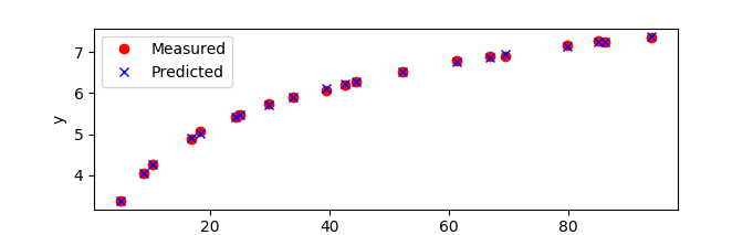
Example: Nonlinear Regression
from gekko import GEKKO
# load data
xm = np.array([18.3447,79.86538,85.09788,10.5211,44.4556, \
69.567,8.960,86.197,66.857,16.875, \
52.2697,93.917,24.35,5.118,25.126, \
34.037,61.4445,42.704,39.531,29.988])
ym = np.array([5.072,7.1588,7.263,4.255,6.282, \
6.9118,4.044,7.2595,6.898,4.8744, \
6.5179,7.3434,5.4316,3.38,5.464, \
5.90,6.80,6.193,6.070,5.737])
# define GEKKO model
m = GEKKO()
# parameters and variables
a = m.FV(value=0)
b = m.FV(value=0)
c = m.FV(value=0,lb=-100,ub=100)
x = m.Param(value=xm)
ymeas = m.Param(value=ym)
ypred = m.Var()
# parameter and variable options
a.STATUS = 1 # available to optimizer
b.STATUS = 1 # to minimize objective
c.STATUS = 1
# equation
m.Equation(ypred == a + b/x + c*m.log(x))
# objective
m.Minimize(((ypred-ymeas)/ymeas)**2)
# application options
m.options.IMODE = 2 # regression mode
# solve
m.solve() # remote=False for local solve
# show final objective
print('Final SSE Objective: ' + str(m.options.objfcnval))
# print solution
print('Solution')
print('a = ' + str(a.value[0]))
print('b = ' + str(b.value[0]))
print('c = ' + str(c.value[0]))
# plot solution
import matplotlib.pyplot as plt
plt.figure(1)
plt.plot(x,ymeas,'ro')
plt.plot(x,ypred,'bx');
plt.xlabel('x')
plt.ylabel('y')
plt.legend(['Measured','Predicted'],loc='best')
plt.savefig('results.png')
plt.show()
See also Energy Price Nonlinear Regression