Graphical Method: Second Order Underdamped
 |  | |  |  |
|---|
The objective of these exercises is to fit parameters to describe a second order underdamped system. A second order system differential equation has an output `y(t)`, input `u(t)` and four unknown parameters. The four parameters are the gain `K_p`, damping factor `\zeta`, second order time constant `\tau_s`, and dead time `\theta_p`.
$$\tau_s^2 \frac{d^2y}{dt^2} + 2 \zeta \tau_s \frac{dy}{dt} + y = K_p \, u\left(t-\theta_p \right)$$
The second order system can also be expressed in Laplace-domain form.
$$\frac{Y(s)}{U(s)} = \frac{K_p}{\tau_s^2 s^2 + 2 \zeta \tau_s s + 1}e^{-\theta_p s}$$
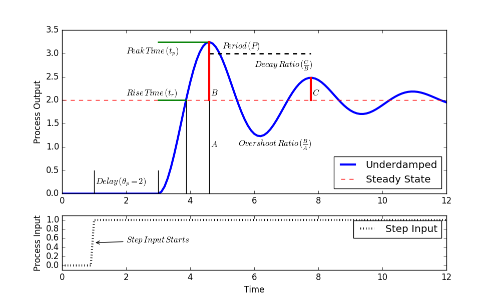
Where applicable, follow the steps to obtain a graphical approximation of a step response of an underdamped (oscillating) second order system. An underdamped system implies that `0 \ge \zeta > 1`.
- Find `\Delta y` from step response.
- Find `\Delta u` from step response.
- Calculate `K_p = {\Delta y} / {\Delta u}`.
- Calculate damping factor `\zeta` from overshoot `OS` or decay ratio `DR`.
- Calculate `\tau_s` from equations for rise time `t_r`, peak time `t_p`, or period `P`.
See Second Order Graphical Methods for additional details on correlations for obtaining the unknown 2nd order system parameters. Assume a step input of 1.0 for each output graph for Exercises 1a-1c.
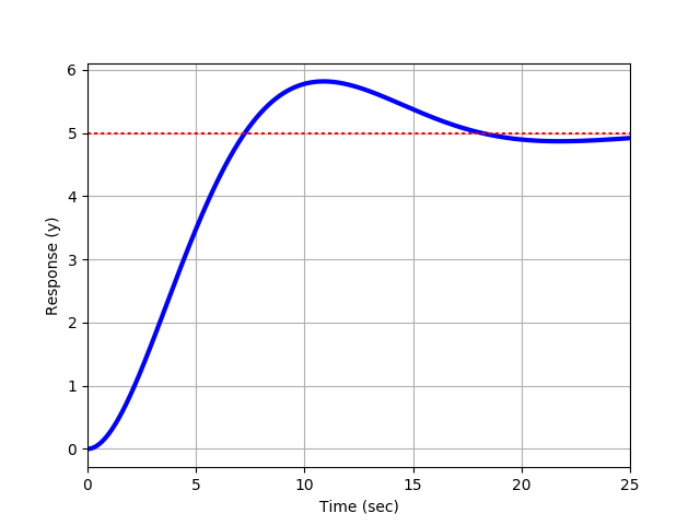
Exercise 1a
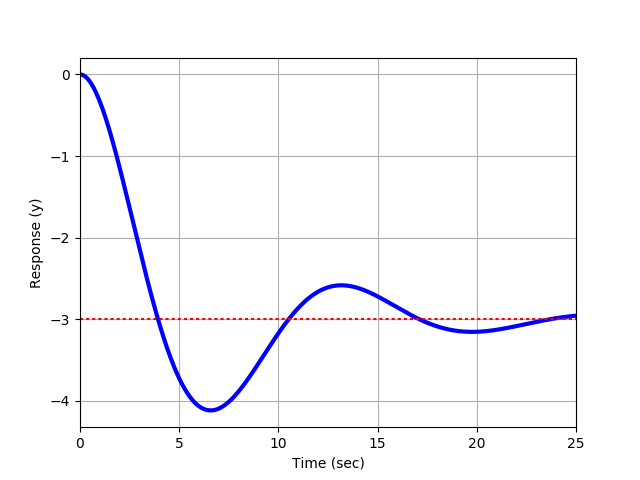
Exercise 1b
Exercise 1c
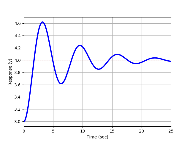
Use the following script to generate a step response for a 2nd order system. For each of the exercises (1a-1c), you can plug in the values for `K_p`, `\tau_s`, and zeta (`\zeta`) to generate a step response.
from scipy import signal
import matplotlib.pyplot as plt
from scipy.integrate import odeint
# Change these values based on graphical fit
Kp = 1.0
taus = 1.0
zeta = 1.0
# Transfer Function
# Kp / (taus * s**2 + 2 * zeta * taus * s + 1)
num = [Kp]
den = [taus**2,2.0*zeta*taus,1]
sys1 = signal.TransferFunction(num,den)
t1,y1 = signal.step(sys1)
plt.figure(1)
plt.plot(t1,y1,'b--',linewidth=3,label='Transfer Fcn')
plt.xlabel('Time')
plt.ylabel('Response (y)')
plt.legend(loc='best')
plt.show()
Exercise 2
A PI closed loop controller process variable (PV) rises to meet a new set point (SP) following a change from 50 to 70. The PV overshoots the new set point by 50% with two success peak values at 100 and 300 seconds after the set point change is initiated. The PV response eventually settles to the new SP with no offset. Determine the gain `K_p`, damping factor `\zeta`, and second order time constant `\tau_s` that describe the closed loop response as a second order underdamped system. Assume that dead time `\theta_p` is negligible.
What to Turn In
- Exercises 1a-1c: Graphical estimation of Kₚ, ζ, τₛ, and θₚ from the plotted step response. Show how each parameter was determined from the graph.
- Exercise 2: Determine Kₚ, ζ, and τₛ that describe the PI-controlled process. Show supporting calculations based on overshoot, decay ratio, and peak timing. Include a summary of how these parameters characterize the closed-loop system response.