Dynamics and Control

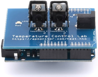
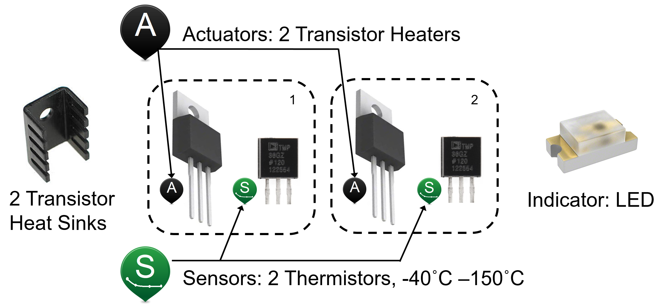
Objective: Derive and simulate a state space model for two heaters and compare the model predictions with the Arduino temperature control lab measurements.

A TCLab state space model is a linear representation of the physics-based model. Putting a model into state space form is the basis for many methods in process dynamics and control analysis and will be used for model predictive control in a later exercise.

A physics-based model is developed in prior exercises. A 2nd-order physics-based model consists of four differential equations from energy balances that include convection, conduction, and thermal radiation.

$$m\,c_p\frac{dT_{H1}}{dt} = U\,A\,\left(T_\infty-T_{H1}\right) + \epsilon\,\sigma\,A\,\left(T_\infty^4-T_{H1}^4\right) + Q_{C12} + Q_{R12} + \alpha_1 Q_1$$

$$m\,c_p\frac{dT_{H2}}{dt} = U\,A\,\left(T_\infty-T_{H2}\right) + \epsilon\,\sigma\,A\,\left(T_\infty^4-T_{H2}^4\right) - Q_{C12} - Q_{R12} + \alpha_2 Q_2$$

$$\tau \frac{dT_{C1}}{dt} = T_{H1} - T_{C1}$$

$$\tau \frac{dT_{C2}}{dt} = T_{H2} - T_{C2}$$

with the following heat transfer terms for simplifying the expressions.

$$Q_{C12} = U_s \, A_s \, \left(T_{H2}-T_{H1}\right)$$

$$Q_{R12} = \epsilon\,\sigma\,A_s\,\left(T_{H2}^4-T_{H1}^4\right)$$

$$\tau = \frac{m_s \, c_{p,s} \, \Delta x}{k\,A_c}$$

Use these equations to develop a state space model of the temperature response to heater changes.

$$\begin{bmatrix}\dot T'_{H1}\\\dot T'_{H2}\\\dot T'_{C1}\\\dot T'_{C2}\end{bmatrix} = \begin{bmatrix}a_{1,1} & a_{1,2} & a_{1,3} & a_{1,4}\\a_{2,1} & a_{2,2} & a_{2,3} & a_{2,4}\\a_{3,1} & a_{3,2} & a_{3,3} & a_{3,4}\\a_{4,1} & a_{4,2} & a_{4,3} & a_{4,4}\end{bmatrix} \begin{bmatrix}T'_{H1}\\T'_{H2}\\T'_{C1}\\T'_{C2}\end{bmatrix} + \begin{bmatrix}b_{1,1} & b_{1,2}\\b_{2,1} & b_{2,2}\\b_{3,1} & b_{3,2}\\b_{4,1} & b_{4,2}\end{bmatrix} \begin{bmatrix}Q'_1\\Q'_2\end{bmatrix}$$

$$\begin{bmatrix}T'_{C1}\\T'_{C2}\end{bmatrix} = \begin{bmatrix}0 & 0 & 1 & 0\\0 & 0 & 0 & 1\end{bmatrix} \begin{bmatrix}T'_{H1}\\T'_{H2}\\T'_{C1}\\T'_{C2}\end{bmatrix} + \begin{bmatrix}0&0\\0&0\end{bmatrix} \begin{bmatrix}Q'_1\\Q'_2\end{bmatrix}$$

This state space model:

$$\dot x = A x + B u$$

$$y = C x + D u$$

has four matrices with `A` and `B` that need to be obtained from partial derivatives of the right hand side of the differential equations.

$$A \in \mathbb{R}^{4 \, \mathrm{x} \, 4} = \begin{bmatrix}a_{1,1} & a_{1,2} & a_{1,3} & a_{1,4}\\a_{2,1} & a_{2,2} & a_{2,3} & a_{2,4}\\a_{3,1} & a_{3,2} & a_{3,3} & a_{3,4}\\a_{4,1} & a_{4,2} & a_{4,3} & a_{4,4}\end{bmatrix}$$ $$B \in \mathbb{R}^{4 \, \mathrm{x} \, 2} = \begin{bmatrix}b_{1,1} & b_{1,2}\\b_{2,1} & b_{2,2}\\b_{3,1} & b_{3,2}\\b_{4,1} & b_{4,2}\end{bmatrix} $$ $$C \in \mathbb{R}^{2 \, \mathrm{x} \, 4} = \begin{bmatrix}0 & 0 & 1 & 0\\0 & 0 & 0 & 1\end{bmatrix}$$ $$D \in \mathbb{R}^{2 \, \mathrm{x} \, 2} = \begin{bmatrix}0&0\\0&0\end{bmatrix}$$

The individual elements are obtained by evaluating partial derivatives of the differential equations at steady state conditions.

$$a_{1,1} = \frac{\partial f_1}{\partial T_{H1}}\bigg|_{\bar T} = -\frac{U\,A + 4 \epsilon \sigma A T_0^3 + U_s \, A_s + 4 \epsilon \sigma A_s T_0^3}{m\,C_p}$$

$$a_{1,2} = \frac{\partial f_1}{\partial T_{H2}}\bigg|_{\bar T} = \frac{U_s \, A_s + 4 \epsilon \sigma A_s T_0^3}{m\,C_p}$$

Fill in the values of the state space matrices after the parameters (U, U_s, `\tau`, `\alpha_1`, and `\alpha_2`) are estimated.

Add a simulation of the linear model with either Gekko or Scipy with the same heater inputs as used during the test.

Simulate Linear Model Am, Bm, Cm, Dm with Gekko

Simulate Linear Model Am, Bm, Cm, Dm with Scipy

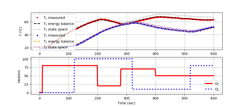
Add the predictions to the plot by adding the nominal temperature (T₀=21^oC) to the output to return to ^oC from deviation variable form.

Solution

import numpy as np
import matplotlib.pyplot as plt
import pandas as pd
from gekko import GEKKO
import tclab
import time
from scipy import signal

# Import data
try:
    # try to read local data file first
    filename = 'data.csv'
    data = pd.read_csv(filename)
except:
    # heater steps
    Q1d = np.zeros(601)
    Q1d[10:200] = 80
    Q1d[200:280] = 20
    Q1d[280:400] = 70
    Q1d[400:] = 50

    Q2d = np.zeros(601)
    Q2d[120:320] = 100
    Q2d[320:520] = 10
    Q2d[520:] = 80

    try:
        # Connect to Arduino
        a = tclab.TCLab()
        fid = open(filename,'w')
        fid.write('Time,Q1,Q2,T1,T2\n')
        fid.close()

        # run step test (10 min)
        for i in range(601):
            # set heater values
            a.Q1(Q1d[i])
            a.Q2(Q2d[i])
            print('Time: ' + str(i) + \
                  ' Q1: ' + str(Q1d[i]) + \
                  ' Q2: ' + str(Q2d[i]) + \
                  ' T1: ' + str(a.T1)   + \
                  ' T2: ' + str(a.T2))
            # wait 1 second
            time.sleep(1)
            fid = open(filename,'a')
            fid.write(str(i)+','+str(Q1d[i])+','+str(Q2d[i])+',' \
                      +str(a.T1)+','+str(a.T2)+'\n')
        # close connection to Arduino
        a.close()
        fid.close()
    except:
        filename = 'https://apmonitor.com/pdc/uploads/Main/tclab_data2.txt'
    # read either local file or use link if no TCLab
    data = pd.read_csv(filename)

# Fit Parameters of Energy Balance
m = GEKKO() # Create GEKKO Model

# Parameters to Estimate
U = m.FV(value=10,lb=1,ub=20)
Us = m.FV(value=20,lb=5,ub=40)
alpha1 = m.FV(value=0.01,lb=0.001,ub=0.03)  # W / % heater
alpha2 = m.FV(value=0.005,lb=0.001,ub=0.02) # W / % heater
tau = m.FV(value=10.0,lb=5.0,ub=60.0)

# Measured inputs
Q1 = m.Param()
Q2 = m.Param()

Ta =21.0+273.15                     # K
mass = 4.0/1000.0                   # kg
Cp = 0.5*1000.0                     # J/kg-K    
A = 10.0/100.0**2                   # Area not between heaters in m^2
As = 2.0/100.0**2                   # Area between heaters in m^2
eps = 0.9                           # Emissivity
sigma = 5.67e-8                     # Stefan-Boltzmann

TH1 = m.SV()
TH2 = m.SV()
TC1 = m.CV()
TC2 = m.CV()

# Heater Temperatures in Kelvin
T1 = m.Intermediate(TH1+273.15)
T2 = m.Intermediate(TH2+273.15)

# Heat transfer between two heaters
Q_C12 = m.Intermediate(Us*As*(T2-T1)) # Convective
Q_R12 = m.Intermediate(eps*sigma*As*(T2**4-T1**4)) # Radiative

# Energy balances
m.Equation(TH1.dt() == (1.0/(mass*Cp))*(U*A*(Ta-T1) \
                + eps * sigma * A * (Ta**4 - T1**4) \
                + Q_C12 + Q_R12 \
                + alpha1*Q1))

m.Equation(TH2.dt() == (1.0/(mass*Cp))*(U*A*(Ta-T2) \
                + eps * sigma * A * (Ta**4 - T2**4) \
                - Q_C12 - Q_R12 \
                + alpha2*Q2))

# Conduction to temperature sensors
m.Equation(tau*TC1.dt() == TH1-TC1)
m.Equation(tau*TC2.dt() == TH2-TC2)

# Options
# STATUS=1 allows solver to adjust parameter
U.STATUS = 1  
Us.STATUS = 1  
alpha1.STATUS = 1
alpha2.STATUS = 1
tau.STATUS = 1

Q1.value=data['Q1'].values
Q2.value=data['Q2'].values
TH1.value=data['T1'].values[0]
TH2.value=data['T2'].values[0]
TC1.value=data['T1'].values
TC1.FSTATUS = 1    # minimize fstatus * (meas-pred)^2
TC2.value=data['T2'].values
TC2.FSTATUS = 1    # minimize fstatus * (meas-pred)^2

m.time = data['Time'].values
m.options.IMODE   = 5 # MHE
m.options.EV_TYPE = 2 # Objective type
m.options.NODES   = 2 # Collocation nodes
m.options.SOLVER  = 3 # IPOPT

m.solve(disp=False) # Solve physics-based model

# Parameter values
print('Estimated Parameters')
print('U     : ' + str(U.value[0]))
print('Us     : ' + str(Us.value[0]))
print('alpha1: ' + str(alpha1.value[0]))
print('alpha2: ' + str(alpha2.value[-1]))
print('tau: ' + str(tau.value[0]))

print('Constants')
print('Ta: ' + str(Ta))
print('m: ' + str(mass))
print('Cp: ' + str(Cp))
print('A: ' + str(A))
print('As: ' + str(As))
print('eps: ' + str(eps))
print('sigma: ' + str(sigma))

Am = np.zeros((4,4))
Bm = np.zeros((4,2))
Cm = np.zeros((2,4))
Dm = np.zeros((2,2))

T0 = Ta
c1 = U.value[0]*A
c2 = 4*eps*sigma*A*T0**3
c3 = Us.value[0]*As
c4 = 4*eps*sigma*As*T0**3
c5 = mass*Cp
c6 = 1/tau.value[0]

Am[0,0] = -(c1+c2+c3+c4)/c5
Am[0,1] = (c3+c4)/c5

Am[1,0] = (c3+c4)/c5
Am[1,1] = -(c1+c2+c3+c4)/c5

Am[2,0] = c6
Am[2,2] = -c6

Am[3,1] = c6
Am[3,3] = -c6

Bm[0,0] = alpha1.value[0]/c5
Bm[1,1] = alpha2.value[0]/c5

Cm[0,2] = 1
Cm[1,3] = 1

# state space simulation
ss = GEKKO()
x,y,u = ss.state_space(Am,Bm,Cm,D=None)
u[0].value = data['Q1'].values
u[1].value = data['Q2'].values
ss.time = data['Time'].values
ss.options.IMODE = 7
ss.solve(disp=False)

# state space simulation with scipy
sys = signal.StateSpace(Am,Bm,Cm,Dm)
tsys = data['Time'].values
Qsys = np.vstack((data['Q1'].values,data['Q2'].values))
Qsys = Qsys.T
tsys,ysys,xsys = signal.lsim(sys,Qsys,tsys)

sae = 0.0
for i in range(len(data)):
    sae += np.abs(data['T1'][i]-TC1.value[i])
    sae += np.abs(data['T2'][i]-TC2.value[i])
print('SAE Energy Balance: ' + str(sae))

# Create plot
plt.figure(figsize=(10,7))
ax=plt.subplot(2,1,1)
ax.grid()
plt.plot(data['Time'],data['T1'],'r.',label=r'$T_1$ measured')
plt.plot(m.time,TC1.value,color='black',linestyle='--',\
         linewidth=2,label=r'$T_1$ energy balance')
plt.plot(ss.time,np.array(y[0].value)+21.0,color='gray',linestyle=':',\
         linewidth=2,label=r'$T_1$ state space')
plt.plot(data['Time'],data['T2'],'b.',label=r'$T_2$ measured')
plt.plot(m.time,TC2.value,color='orange',linestyle='--',\
         linewidth=2,label=r'$T_2$ energy balance')
plt.plot(ss.time,np.array(y[1].value)+21.0,color='purple',linestyle=':',\
         linewidth=2,label=r'$T_2$ state space')
plt.ylabel(r'T ($^oC$)')
plt.legend(loc=2)
ax=plt.subplot(2,1,2)
ax.grid()
plt.plot(data['Time'],data['Q1'],'r-',\
         linewidth=3,label=r'$Q_1$')
plt.plot(data['Time'],data['Q2'],'b:',\
         linewidth=3,label=r'$Q_2$')
plt.ylabel('Heaters')
plt.xlabel('Time (sec)')
plt.legend(loc='best')
plt.savefig('tclab_state_space.png')
plt.show()

[$[Get Code]]