State Space Stirred Reactor
 |  |  |  |
|---|
The exercise involves creating a dynamic model based on balance equations, linearizing, and putting the equations into state space form. A reactor is used to convert a hazardous chemical A to an acceptable chemical B in waste stream before entering a nearby lake. This particular reactor is dynamically modeled as a Continuously Stirred Tank Reactor (CSTR) with a simplified kinetic mechanism that describes the conversion of reactant A to product B with an irreversible and exothermic reaction.
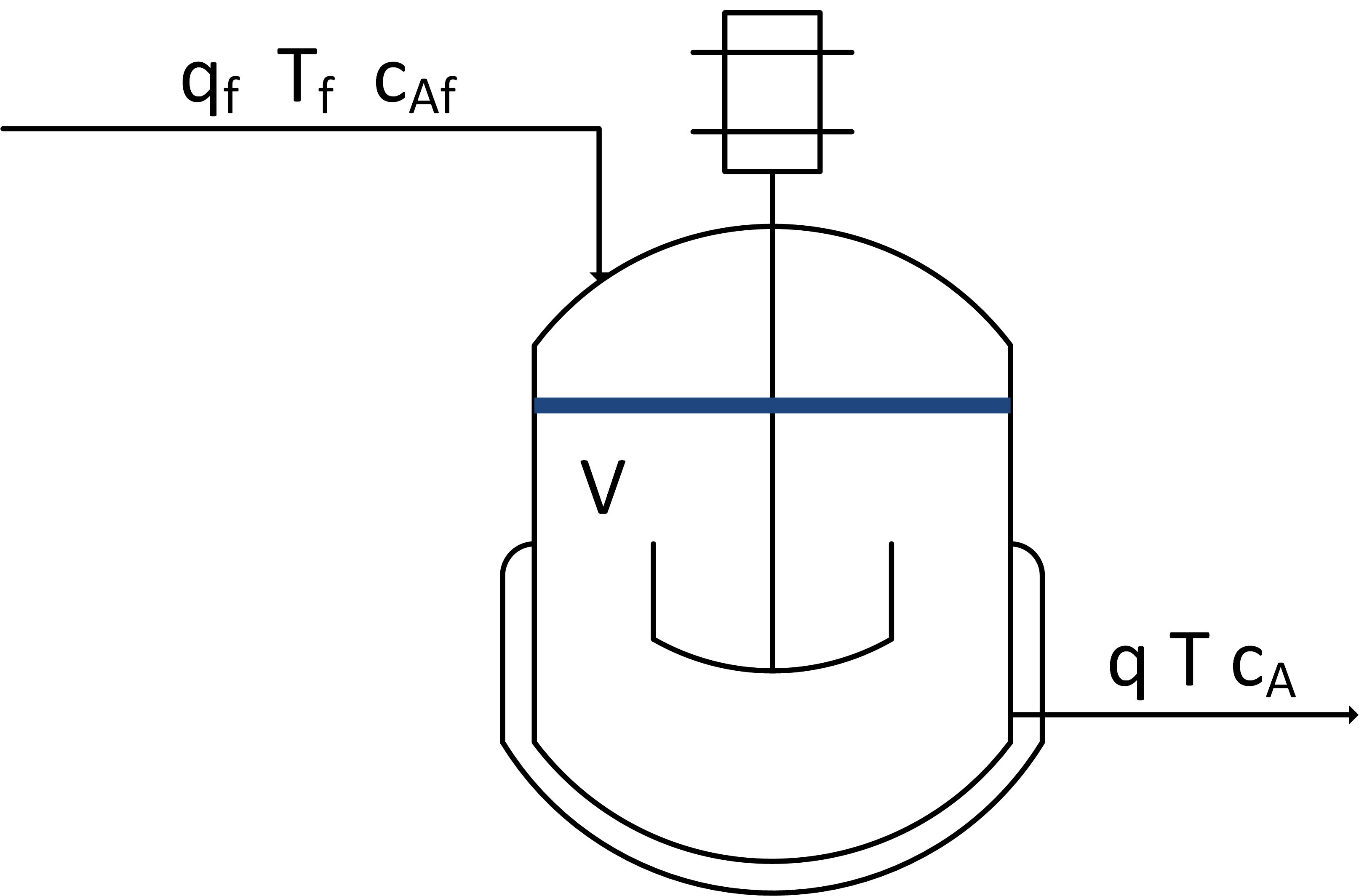
Linearize species and energy balances that describe the dynamic response in concentration and temperature of a well-mixed vessel with constant volume V = 10 m3, volumetric flow q = 5 m3/min, feed temperature Tf = 300 K, initial concentration Ca0 = 0.5 mol/L, and initial temperature T0 = 305 K. The chemical A is converted to chemical B with first order reaction kinetics rA = 0.5 Ca. The reaction is exothermic with a heat of reaction of 10 J/mol. The following species and energy balances represent the reactor concentration and temperature.
$$\frac{dC_a}{dt} = \frac{q}{V} \left(C_{af} - C_a \right) - r_A$$
$$\frac{dT}{dt} = \frac{q}{V} \left(T_f-T\right) + \Delta H_r \; r_A$$
See model simulation help for information on simulating transfer function, state space, and general nonlinear models. Put the resulting model into state space form by filling in following numbers of the starting script.
A[0,0] = ### fill-in value ###
B[0,0] = ### fill-in value ###
A[1,0] = ### fill-in value ###
A[1,1] = ### fill-in value ###
import matplotlib.pyplot as plt
from scipy.integrate import odeint
from scipy import signal
# define linear model
# Inputs (u)
# u[0] = Caf
# u[1] = Tf
# States and Outputs (x,y)
# x[0] = y[0] = Ca
# x[1] = y[1] = T
# dx/dt = A * x + B * u
# y = C * x + D * u
# Equations
# rA = 0.5 * Ca
# Hr = 10
# V * dCa/dt = qf*Caf - q*Ca - rA*V
# V * dT/dt = qf*Tf - q*T + Hr*rA*V
# Simplified Equations
# dCa/dt = 0.5*(Caf - Ca) - 0.5*Ca
# dT/dt = 0.5*(Tf - T) + 5.0*Ca
# State Space Matrices
n = 2
m = 1
p = 2
A = np.zeros((n,n))
B = np.zeros((n,m))
# Linearized equation non-zero elements
A[0,0] = ### fill-in value ###
B[0,0] = ### fill-in value ###
A[1,0] = ### fill-in value ###
A[1,1] = ### fill-in value ###
# Define outputs
C = np.eye(n)
D = np.zeros((p,m))
# Define state space model
sys = signal.StateSpace(A,B,C,D)
# Step of 1.0 to 10 min
t = np.linspace(0,10,101)
t_sys,y_sys = signal.step(sys,T=t)
# Step of -0.1
y_sys = -0.1 * y_sys
# Add steady state values
Ca0 = 0.5
T0 = 305.0
Ca_sys = y_sys[:,0] + Ca0
T_sys = y_sys[:,1] + T0
# define reactor model
def reactor(x,t,Caf):
# Inputs (2):
# Caf = Feed Concentration (mol/L)
# Tf = Feed Temperature (K)
# States (2):
# Concentration of A (mol/L)
Ca = x[0]
# Temperature (K)
T = x[1]
# Parameters:
rA = 0.5 * Ca
Hr = 10
V = 10.0
q = 5.0
Tf = 300.0
# Species balance: concentration derivative
dCadt = q*(Caf - Ca)/V - rA
# Energy balance: temperature derivative
dTdt = q*(Tf - T)/V + Hr * rA
# Return derivatives
return [dCadt,dTdt]
# Initial Conditions
y0 = [Ca0,T0]
# Feed Concentration (mol/L)
Caf = np.ones(len(t))*1.0
Caf[0:] = 0.9
# Storage for results
Ca = np.ones(len(t))*Ca0
T = np.ones(len(t))*T0
# Loop through each time step
for i in range(len(t)-1):
# Simulate
inputs = (Caf[i],)
ts = [t[i],t[i+1]]
y = odeint(reactor,y0,ts,args=inputs)
# Store results
Ca[i+1] = y[-1][0]
T[i+1] = y[-1][1]
# Adjust initial condition for next loop
y0 = y[-1]
# Construct results and save data file
data = np.vstack((t,Caf,Ca,T)) # vertical stack
data = data.T # transpose data
np.savetxt('data.txt',data,delimiter=',')
# Plot the inputs and results
plt.figure()
plt.subplot(3,1,1)
Caf[0] = 1.0
plt.plot(t,Caf,'k-',label='Caf')
plt.legend(loc='best')
plt.subplot(3,1,2)
plt.plot(t,Ca,'r-',label='Ca')
plt.plot(t_sys,Ca_sys,'b--',label='Ca (State Space)')
plt.legend(loc='best')
plt.subplot(3,1,3)
plt.plot(t,T,'r-',label='T')
plt.plot(t_sys,T_sys,'b--',label='T (State Space)')
plt.legend(loc='best')
plt.xlabel('Time (min)')
plt.show()
Compare the state space model response to the numerical integration shown below with a step changes Caf from 1.0 mol/L to 0.9 mol/L. Fill in the A and B state space matrices in the Python script.