Deploy Machine Learning
Training and testing are often performed once on a dedicated computing platform. The trained model is then packaged for another computing system for predictions. An example of this training and deployment is the Tesla Autopilot as demonstrated in the Tesla AI Day.
Deploying machine learning is the process of making the model available to produce results for people or computers to access the model predictions. It involves managing data flow to the application for training or prediction. Data flow can be in batches or a continuous stream.

The machine learning application may be deployed in many ways such as through an Application Programming Interface (API), a web-interface, an APP for mobile devices, or through a Jupyter Notebook or Python script. A few exercises demonstrate packaging and transfer of applications for deployment.


If the machine learned model is trained offline, the model is encapsulated and transferred to the hosting target. A scalable deployment means that the computing architecture can handle increased demand such as through a cloud computing host with on-demand scale-up. A Docker container can be deployed to cloud services.
Pickle Files

Pickle files store Python objects, lists of objects, or anything else that is accessible in a Python session. The list z is dumped to the Pickle file z.pkl.
import pickle
pickle.dump(z,open('z.pkl','wb'))
The z.pkl can then be accessed later on that same computer or transferred to another computer and loaded.
y = pickle.load(open('z.pkl','rb'))
print(y)
HDF5 Files

Some Python objects, such as Keras models, cannot be stored as Pickle files. The Hierarchical Data Format, version 5 (HDF5) is a file format that is designed to store large amounts of data, model architecture, parameter weights, and other information about machine learned models. Keras supports model save and load in HDF5 format (see Keras documentation).
Save HDF5 Model
The Keras model is saved with:
- Keras / TensorFlow model architecture (layers, nodes, connections) and configuration (hyper-parameters such as lbfgs or adam solver, loss function, epochs, early termination criteria)
- Weights that are adjusted during training and used for testing and validation
Load HDF5 Model
model = load_model('store.h5')
The model is restored into the running program by calling load_model to read the hdf5 file and rebuilt the Keras model to perform testing, validation, or deploy the machine learning solution. Concrete Image Classification demonstrates TensorFlow training with an h5 file that transfers the model to the test program.
 TensorFlow Model cracks.h5 is Retrieved
import re
import random
import numpy as np
import os
import zipfile
import urllib.request
import matplotlib.pyplot as plt
from tensorflow.keras.preprocessing import image
from tensorflow.keras.preprocessing.image import ImageDataGenerator
from tensorflow import keras
# download cracks.h5 (TensorFlow model)
file = 'cracks.h5'
url = 'http://apmonitor.com/pds/uploads/Main/'+file
urllib.request.urlretrieve(url, file)
# download concrete_cracks.zip (Images)
file = 'concrete_cracks.zip'
url = 'http://apmonitor.com/pds/uploads/Main/'+file
urllib.request.urlretrieve(url, file)
# extract archive and remove concrete_cracks.zip
with zipfile.ZipFile(file, 'r') as zip_ref:
zip_ref.extractall('./')
os.remove(file)
# Data processing
test_processor = ImageDataGenerator(rescale = 1./255)
test = test_processor.flow_from_directory('test', \
target_size = (128, 128), batch_size = 32, \
class_mode = 'categorical', shuffle = False)
# load the trained model
model = keras.models.load_model('cracks.h5')
ctype = ['Negative','Positive'] # possible output values
def make_prediction(image_fp):
im = cv2.imread(image_fp) # load image
plt.imshow(im)
img = image.load_img(image_fp, target_size = (128,128))
img = image.img_to_array(img)
image_array = img / 255. # scale the image
img_batch = np.expand_dims(image_array, axis = 0)
predicted_value = ctype[model.predict(img_batch).argmax()]
true_value = re.search(r'(Negative)|(Positive)', image_fp)[0]
out = f"""Predicted Crack: {predicted_value}
True Crack: {true_value}
Correct?: {predicted_value == true_value}"""
return out
# randomly select type (2) and image number (19901-20000)
i = random.randint(0,1); j = random.randint(19901,20000)
b = ctype[i]; im = str(j) + '.jpg'
test_image_filepath = r'./test/'+b+'/'+im
print(make_prediction(test_image_filepath))
plt.show()
Deploy Machine Learning: Logistic Regression
Pickle files can be used to store Scikit-learn machine learning models, data, scalars, or other objects needed to deploy an application on a server or other computer.

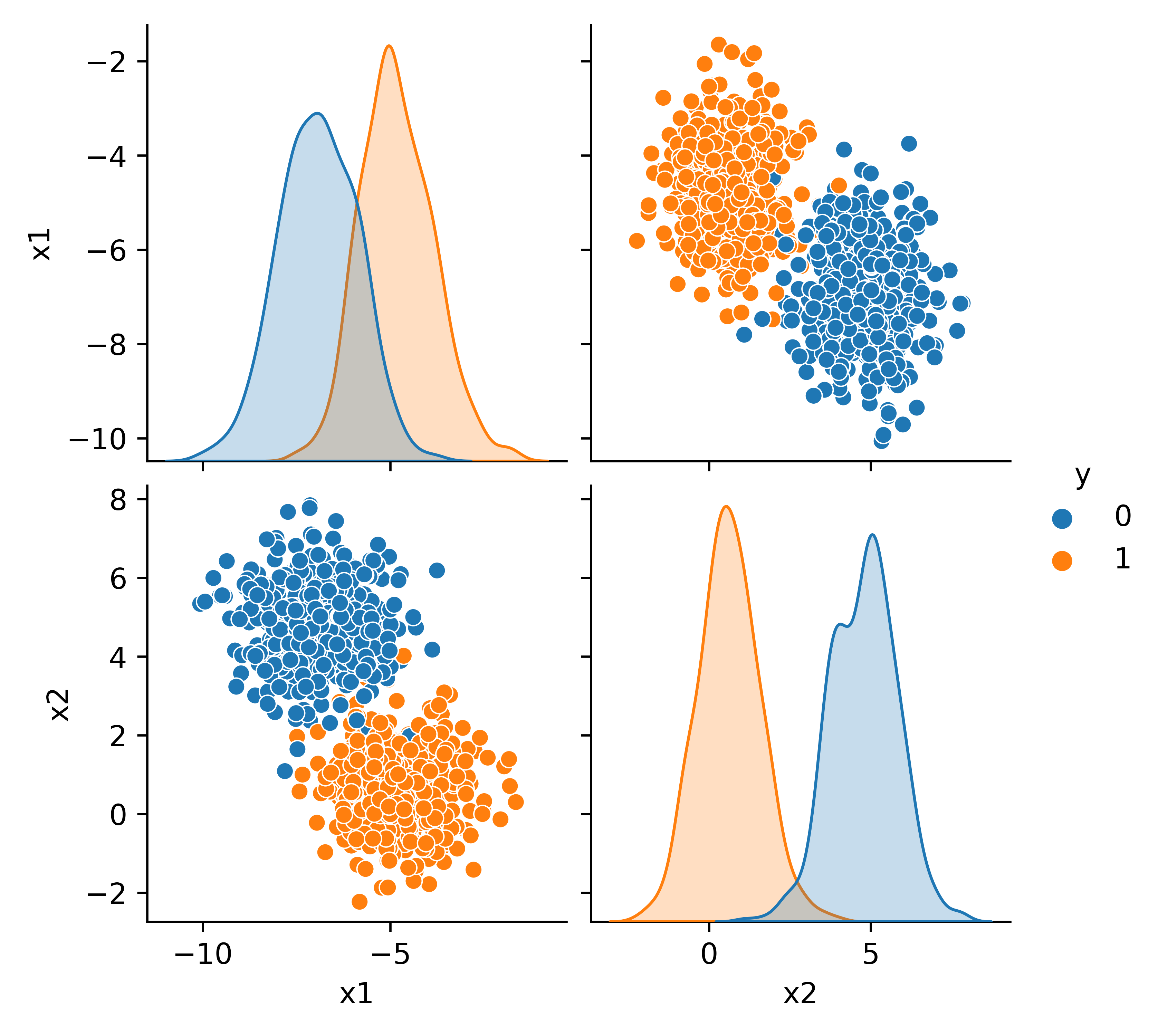
A Logistic Regression model is trained on 800 data points that are randomly generated with the make_blobs function in scikit_learn.
from sklearn.datasets import make_blobs
features, label = make_blobs(n_samples=1000, centers=2,\
n_features=2, random_state=12)
# Split into train and test subsets (20% for test)
from sklearn.model_selection import train_test_split
X_train, X_test, y_train, y_test = train_test_split(
features, label, test_size=0.2, shuffle=False)
# Train Logistic Regression model
from sklearn.linear_model import LogisticRegression
lr = LogisticRegression(solver='lbfgs')
lr.fit(X_train,y_train)
# Store model and test data
import pickle
store = [lr,X_test,y_test]
pickle.dump(store,open('store.pkl','wb'))
# View data
import pandas as pd
import seaborn as sns
import matplotlib.pyplot as plt
data = pd.DataFrame({'x1':features[:,0],
'x2':features[:,1],
'y':label})
sns.pairplot(data,hue='y')
plt.show()
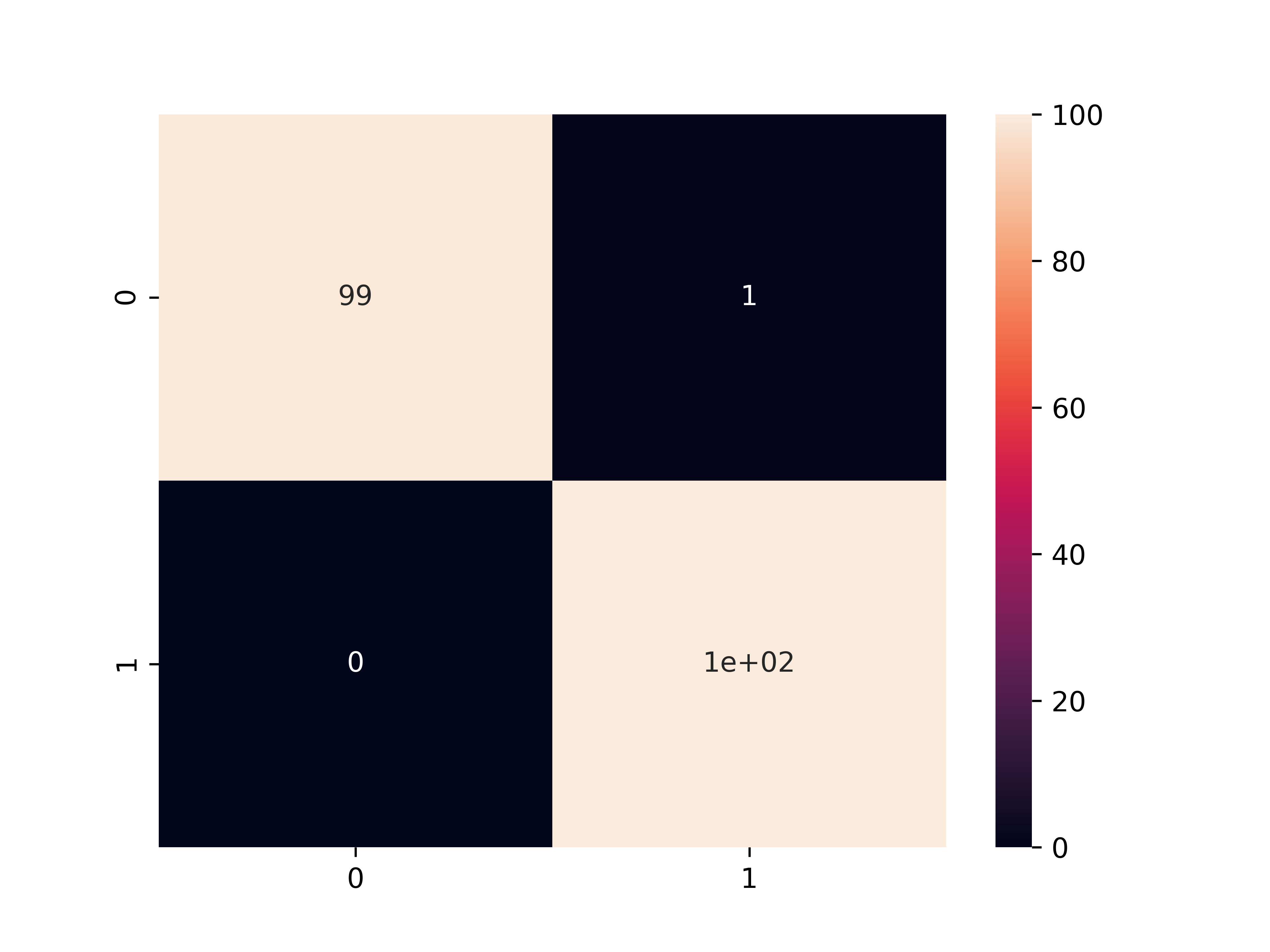
The model and test data are stored in a Pickle file store.pkl. That file can be transferred to another target computer to make predictions.
import pickle
[lr,X_test,y_test] = pickle.load(open('store.pkl','rb'))
# Predict
y_predict = lr.predict(X_test)
# Generate confusion matrix
from sklearn.metrics import confusion_matrix
import seaborn as sns
import matplotlib.pyplot as plt
cmat = confusion_matrix(y_test,y_predict)
sns.heatmap(cmat,annot=True)
plt.show()
Deploy Machine Learning: Number Identification
The next activity is to split a program that includes training and testing into two separate programs. Use a pickle file to store the test data and the neural network model.
Separate machine learning for number identification into a training and test program. Show that the test program can predict the second to last number in the dataset.

from sklearn.model_selection import train_test_split
import matplotlib.pyplot as plt
import numpy as np
from sklearn.neural_network import MLPClassifier
classifier = MLPClassifier(solver='lbfgs',alpha=1e-5,max_iter=200,\
activation='relu',hidden_layer_sizes=(10,30,10),\
random_state=1, shuffle=True)
# The digits dataset
digits = datasets.load_digits()
n_samples = len(digits.images)
data = digits.images.reshape((n_samples, -1))
# Split into train and test subsets (50% each)
X_train, X_test, y_train, y_test = train_test_split(
data, digits.target, test_size=0.5, shuffle=False)
# Learn the digits on the first half of the digits
classifier.fit(X_train, y_train)
# Test on second half of data
n = np.random.randint(int(n_samples/2),n_samples)
print('Predicted: ' + str(classifier.predict(digits.data[n:n+1])[0]))
# Show number
plt.imshow(digits.images[n], cmap=plt.cm.gray_r, interpolation='nearest')
plt.show()
The model and test data are stored in a Pickle file store.pkl.
from sklearn.model_selection import train_test_split
import matplotlib.pyplot as plt
import numpy as np
from sklearn.neighbors import KNeighborsClassifier
classifier = KNeighborsClassifier(n_neighbors=5)
# The digits dataset
digits = datasets.load_digits()
n_samples = len(digits.images)
data = digits.images.reshape((n_samples, -1))
# Split into train and test subsets (50% each)
X_train, X_test, y_train, y_test = train_test_split(
data, digits.target, test_size=0.5, shuffle=False)
# Learn the digits on the first half of the digits
classifier.fit(X_train, y_train)
# Store model and test data
import pickle
store = [classifier,digits]
pickle.dump(store,open('store.pkl','wb'))
That file can be transferred to another target computer to make predictions.
import pickle
[classifier,digits] = pickle.load(open('store.pkl','rb'))
# Test on second to last number
print('Predicted: ' + str(classifier.predict(digits.data[-2:-1])[0]))
# Show number
plt.imshow(digits.images[-2], cmap=plt.cm.gray_r, interpolation='nearest')
plt.show()
Deploy Machine Learning: Gekko MPC
Model Predictive Control (MPC) is an advanced control method to regulate and optimize dynamic systems. MPC uses time-based predictions to make adjustments that meet control objectives. The controller runs at a specified cycle time such as every second or minute. MPC is deployed with a data acquisition system to retrieve current process measurements, reoptimize the move plan, and send commands to acquators. The Gekko package uses combinations of physics-based, time-series, and machine learned models for predictions. The model and options can be stored in a Pickle file (e.g. m.pkl). In this example, the model is rebuilt if the Pickle file does not exist. Otherwise, the Pickle file is loaded and the MPC is solved again to create an updated move plan. Complete MPC instructions are provided with advanced temperature control of the TCLab.
import pickle
import numpy as np
from gekko import GEKKO
import matplotlib.pyplot as plt
if exists('m.pkl'):
# load model from subsequent call
m = pickle.load(open('m.pkl','rb'))
m.solve(disp=False)
else:
# define model the first time
m = GEKKO()
m.time = np.linspace(0,20,41)
m.p = m.MV(value=0, lb=0, ub=1)
m.v = m.CV(value=0)
m.Equation(5*m.v.dt() == -m.v + 10*m.p)
m.options.IMODE = 6
m.p.STATUS = 1; m.p.DCOST = 1e-3
m.v.STATUS = 1; m.v.SP = 40; m.v.TAU = 5
m.options.CV_TYPE = 2
m.solve(disp=False)
pickle.dump(m,open('m.pkl','wb'))
plt.figure()
plt.subplot(2,1,1)
plt.plot(m.time,m.p.value,'b-',lw=2)
plt.ylabel('gas')
plt.subplot(2,1,2)
plt.plot(m.time,m.v.value,'r--',lw=2)
plt.ylabel('velocity')
plt.xlabel('time')
plt.show()
Further Reading
- Docker Docs, Docker Python Language-Specific Guide, Accessed Feb 2022.
- Opeyemi, B., Deployment of Machine Learning Models Demystified: Part 1 and Part 2, Nov 2019.
- Huyen, C., Real-time machine learning: challenges and solutions, Jan 2022.

✅ Knowledge Check
1. Which statement is correct regarding deploying machine learning models?
- Incorrect. Deploying machine learning models is not just about training. It refers to making the model available to produce results so that people or computers can access its predictions. This includes the process of managing data flow to the application, be it for training or prediction.
- Incorrect. This is not true. Often, models are trained on one computing platform and then packaged for deployment on another computing system for predictions. This allows for flexibility and broader application.
- Incorrect. While Pickle files can be used to store machine learning models, they can also be used to store other Python objects, data, scalars, and more.
- Correct. Yes, machine learning applications can be deployed in various ways, including through APIs, web-interfaces, mobile apps, or even Jupyter Notebooks and Python scripts. This ensures that users can interact and access predictions in a way that is most convenient.
2. What is the primary purpose of the HDF5 file format in the context of machine learning?
- Incorrect. While HDF5 is designed to store large amounts of data, in the context of machine learning, it is particularly useful for storing model architecture, parameter weights, and other information about machine learned models. It is not specifically for video files.
- Incorrect. HDF5 and Pickle are different. Some Python objects, such as Keras models, cannot be stored as Pickle files.
- Correct. The HDF5 format is particularly important in machine learning for storing large datasets, the architecture of the model, the weights adjusted during training, and other relevant information.
- Incorrect. While the example provided discusses Keras supporting model save and load in HDF5 format, the HDF5 format itself is not exclusive to Keras and can be used with other libraries and purposes as well.