Linear Regression
Linear regression is a statistical model that is used to predict the value of a continuous dependent variable (the response variable) based on the value of one or more independent variables (the predictor variables). It is based on the assumption that there is a linear relationship between the predictor variables and the response variable.
Regression is the method of adjusting parameters in a model to minimize the difference between the predicted output and the measured output. The predicted output is calculated from a measured input (univariate), multiple inputs and a single output (multiple linear regression), or multiple inputs and outputs (multivariate linear regression).
- linear regression: x and y are scalars
- multiple linear regression: x is a vector, y is a scalar response
- multivariate linear regression: x is a vector, y is a vector response
In machine learning terminology, the data inputs (x) are features and the measured outputs (y) are labels. For a single input and single output, m is the slope and c is the intercept.
$$y=m x + c$$
An alternate way to write this is in matrix form and changing the slope to `\beta_1` and the intercept to `\beta_2`.
$$y = \begin{bmatrix}x&1\end{bmatrix} \begin{bmatrix}m\\c\end{bmatrix} = \begin{bmatrix}x&1\end{bmatrix} \begin{bmatrix}\beta_1\\\beta_2\end{bmatrix}$$
Capital letters are often used to indicate when there are multiple inputs (X) or multiple outputs (Y). The difference between the predicted `X \beta` and measured `Y` output is the error `\epsilon`.
$$Y=X \beta + \epsilon$$
Linear regression analysis determines if the error `\epsilon` has certain statistical properties. For regression, the objective is to minimize the sum of squared errors.
$$J = \min\left(\sum_{i=1}^n \epsilon_i^2\right)$$
The minimum is where the gradient of the objective `\epsilon` is set equal to zero and solved for `\beta`.
$$Y=X \beta$$
Multiply each side by `X^T`
$$X^T Y= X^T X \beta$$
Multiply each side by the inverse of `X^T X` to solve for `\beta`.
$$\beta = \left(X^T X \right)^{-1} X^T Y$$
Although it is possible to solve for the linear regression parameters this way, there are more efficient numerical methods for solving for the regression parameters.
A common requirement is that the errors (residuals) are normally distributed (`N(\mu,\Sigma)`) with zero mean `\mu=0` and covariance `\Sigma`=I (the identity matrix). This implies that the residuals are i.i.d. (independent and identically distributed) random variables. Statistical tests determine if the data fits a linear regression model or if there are unmodeled features of the data that may require a different type of regression model.
Two examples demonstrate multiple Python methods for (1) univariate linear regression and (2) multiple linear regression.
Example 1: Linear Regression
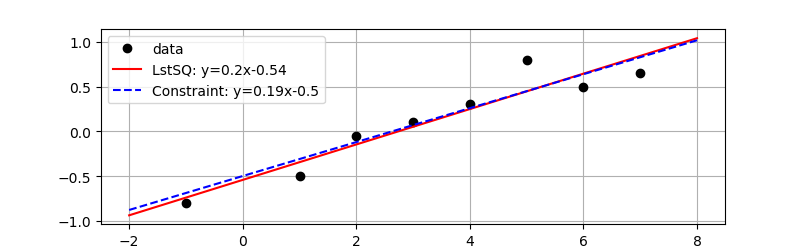
Objective: Perform univariate (single input factor) linear regression on sample data with and without a parameter constraint.
For linear regression, find unknown parameters a0 (slope) and a1 (intercept) to minimize the difference between measured y and predicted yfit.
Data
$$x = [4,5,2,3,-1,1,6,7]$$
$$y = [0.3,0.8,-0.05,0.1,-0.8,-0.5,0.5,0.65]$$
Linear Equation
$$y_{fit} = a_0 x + a_1$$
Minimize Objective
$$\min_{a_0,a_1} \sum_{i=1}^n \left(y_i-y_{fit,i}\right)^2$$
where n is the length of y and a0 and a1 are adjusted to minimize the sum of the squared errors.
Report the parameter values, the R2 value of fit, and display a plot of the results. Enforce a constraint with the intercept>-0.5 and show the effect of that constraint on the regression fit compared to the unconstrained least squares solution.
Solution
There are many methods for regression in Python with 5 different packages to generate the solution. All give the same solution but the methods are different. The methods are from the packages:
- scipy.stats.linregress
- numpy.polyfit
- numpy.linalg
- statsmodels ordinary least squares
- gekko optimization (allows constraints)
============================================================================
Dep. Variable: y R-squared: 0.897
Model: OLS Adj. R-squared: 0.880
Method: Least Squares F-statistic: 52.19
Date: Wed, 26 Aug 2020 Prob (F-statistic): 0.000357
Time: 22:05:45 Log-Likelihood: 2.9364
No. Observations: 8 AIC: -1.873
Df Residuals: 6 BIC: -1.714
Df Model: 1
Covariance Type: nonrobust
============================================================================
coef std err t P>|t| [0.025 0.975]
--------------------------------------------------------------------------
x1 0.1980 0.027 7.224 0.000 0.131 0.265
const -0.5432 0.115 -4.721 0.003 -0.825 -0.262
============================================================================
Omnibus: 2.653 Durbin-Watson: 0.811
Prob(Omnibus): 0.265 Jarque-Bera (JB): 0.918
Skew: 0.827 Prob(JB): 0.632
Kurtosis: 2.862 Cond. No. 7.32
============================================================================
from scipy.stats import linregress
import statsmodels.api as sm
import matplotlib.pyplot as plt
from gekko import GEKKO
# Data
x = np.array([4,5,2,3,-1,1,6,7])
y = np.array([0.3,0.8,-0.05,0.1,-0.8,-0.5,0.5,0.65])
# calculate R^2
def rsq(y1,y2):
yresid= y1 - y2
SSresid = np.sum(yresid**2)
SStotal = len(y1) * np.var(y1)
r2 = 1 - SSresid/SStotal
return r2
# Method 1: scipy linregress
slope,intercept,r,p_value,std_err = linregress(x,y)
a = [slope,intercept]
print('R^2 linregress = '+str(r**2))
# Method 2: numpy polyfit (1=linear)
a = np.polyfit(x,y,1); print(a)
yfit = np.polyval(a,x)
print('R^2 polyfit = '+str(rsq(y,yfit)))
# Method 3: numpy linalg solution
# y = X a
# X^T y = X^T X a
X = np.vstack((x,np.ones(len(x)))).T
# matrix operations
XX = np.dot(X.T,X)
XTy = np.dot(X.T,y)
a = np.linalg.solve(XX,XTy)
# same solution with lstsq
a = np.linalg.lstsq(X,y,rcond=None)[0]
yfit = a[0]*x+a[1]; print(a)
print('R^2 matrix = '+str(rsq(y,yfit)))
# Method 4: statsmodels ordinary least squares
X = sm.add_constant(x,prepend=False)
model = sm.OLS(y,X).fit()
yfit = model.predict(X)
a = model.params
print(model.summary())
# Method 5: Gekko for constrained regression
m = GEKKO(remote=False); m.options.IMODE=2
c = m.Array(m.FV,2); c[0].STATUS=1; c[1].STATUS=1
c[1].lower=-0.5
xd = m.Param(x); yd = m.Param(y); yp = m.Var()
m.Equation(yp==c[0]*xd+c[1])
m.Minimize((yd-yp)**2)
m.solve(disp=False)
c = [c[0].value[0],c[1].value[1]]
print(c)
# plot data and regressed line
plt.plot(x,y,'ko',label='data')
xp = np.linspace(-2,8,100)
slope = str(np.round(a[0],2))
intercept = str(np.round(a[1],2))
eqn = 'LstSQ: y='+slope+'x'+intercept
plt.plot(xp,a[0]*xp+a[1],'r-',label=eqn)
slope = str(np.round(c[0],2))
intercept = str(np.round(c[1],2))
eqn = 'Constraint: y='+slope+'x'+intercept
plt.plot(xp,c[0]*xp+c[1],'b--',label=eqn)
plt.grid()
plt.legend()
plt.show()
Example 2: Multiple Linear Regression
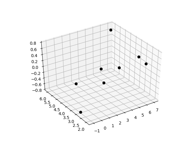
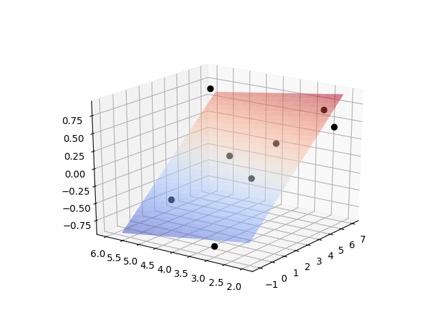
Objective: Perform multiple linear regression on sample data with two inputs.
For linear regression, find unknown parameters a0-a2 to minimize the difference between measured y and predicted yfit.
Data
$$x_0 = [4,5,2,3,-1,1,6,7]$$
$$x_1 = [3,2,3,4, 3,5,2,6]$$
$$y = [0.3,0.8,-0.05,0.1,-0.8,-0.5,0.5,0.65]$$
Linear Equation
$$y_{fit} = a_0 x_0 + a_1 x_1 + a_2$$
Minimize Objective
$$\min_{a_0,a_1} \sum_{i=1}^n \left(y_i-y_{fit,i}\right)^2$$
where n is the length of y and a0-a2 are adjusted to minimize the sum of the squared errors.
Report the parameter values, the R2 value of fit, and display a plot of the results.
Solution
As with univariate linear regression, there are several methods for multiple regression in Python with 3 different packages to generate the solution. Fewer packages in Python can perform multiple or multivariate linear regression. The methods are from the packages:
- numpy.linalg
- statsmodels ordinary least squares
- gekko optimization (allows constraints)
==========================================================================
Dep. Variable: y R-squared: 0.933
Model: OLS Adj. R-squared: 0.906
Method: Least Squares F-statistic: 34.77
Date: Wed, 26 Aug 2020 Prob (F-statistic): 0.00117
Time: 23:16:24 Log-Likelihood: 4.6561
No. Observations: 8 AIC: -3.312
Df Residuals: 5 BIC: -3.074
Df Model: 2
Covariance Type: nonrobust
==========================================================================
coef std err t P>|t| [0.025 0.975]
--------------------------------------------------------------------------
x1 0.2003 0.024 8.256 0.000 0.138 0.263
x2 -0.0750 0.046 -1.639 0.162 -0.193 0.043
const -0.2883 0.186 -1.551 0.182 -0.766 0.190
==========================================================================
Omnibus: 1.262 Durbin-Watson: 1.558
Prob(Omnibus): 0.532 Jarque-Bera (JB): 0.075
Skew: -0.237 Prob(JB): 0.963
Kurtosis: 3.026 Cond. No. 16.9
==========================================================================
import statsmodels.api as sm
from gekko import GEKKO
# Data
x0 = np.array([4,5,2,3,-1,1,6,7])
x1 = np.array([3,2,3,4, 3,5,2,6])
y = np.array([0.3,0.8,-0.05,0.1,-0.8,-0.5,0.5,0.65])
# calculate R^2
def rsq(y1,y2):
yresid= y1 - y2
SSresid = np.sum(yresid**2)
SStotal = len(y1) * np.var(y1)
r2 = 1 - SSresid/SStotal
return r2
# Method 1: numpy linalg solution
# Y = X a
# X^T Y = X^T X a
X = np.vstack((x0,x1,np.ones(len(x0)))).T
a = np.linalg.lstsq(X,y)[0]; print(a)
yfit = a[0]*x0+a[1]*x1+a[2]
print('R^2 = '+str(rsq(y,yfit)))
# Method 2: statsmodels ordinary least squares
model = sm.OLS(y,X).fit()
predictions = model.predict(X)
print(model.summary())
# Method 3: gekko
m = GEKKO(remote=False); m.options.IMODE=2
c = m.Array(m.FV,3)
for ci in c:
ci.STATUS=1
xd = m.Array(m.Param,2); xd[0].value=x0; xd[1].value=x1
yd = m.Param(y); yp = m.Var()
s = m.sum([c[i]*xd[i] for i in range(2)])
m.Equation(yp==s+c[-1])
m.Minimize((yd-yp)**2)
m.solve(disp=False)
a = [c[i].value[0] for i in range(3)]
print(a)
# plot data
from mpl_toolkits import mplot3d
from matplotlib import cm
import matplotlib.pyplot as plt
fig = plt.figure()
ax = plt.axes(projection='3d')
ax.plot3D(x0,x1,y,'ko')
x0t = np.arange(-1,7,0.25)
x1t = np.arange(2,6,0.25)
X0,X1 = np.meshgrid(x0t,x1t)
Yt = a[0]*X0+a[1]*X1+a[2]
ax.plot_surface(X0,X1,Yt,cmap=cm.coolwarm,alpha=0.5)
plt.show()
- Dep. Variable: Model output
- Model: Regression model (OLS=Ordinary Least Squares)
- Method: Regression method
- Date/Time: Time stamp
- No. Observations: Number of data points
- DF Residuals: Residual degrees of freedom. Number of data points – number of parameters
- DF Model: Number of parameters but not including the constant term (intercept)
- R-squared: Coefficient of determination (0-1) is a statistical measure the regression line closeness to the data points (1=perfect alignment)
- Adj. R-squared: Adjusted R-squared based on the number of data points and DF Residuals
- F-statistic: Significance of the fit
- Prob (F-statistic): Probability of the F-statistic
- Log-likelihood: log of the likelihood function
- AIC: Akaike Information Criterion
- BIC: Bayesian Information Criterion
- coef: the regression coefficient
- std err: standard error of the estimated coefficient
- t: t-statistic value that is a measure of the cofficient signficance
- P > |t|: P-value, if less than the confidence level (typically 0.05) the coefficient is a statistically significant in predicting the output
- [0.025 0.975]: 95% confidence interval coefficient bounds
- Skewness: measure of data symmetry. With |skewness|>1 data is highly skewed. If |skewness|<0.5 the data is approximately symmetric.
- Kurtosis: shape of the distribution that compares data at the center with the tails. Data sets with high kurtosis have heavy tails or more outliers. Data sets with low kurtosis have fewer outliers. Kurtosis is 3 for a normal distribution.
- Omnibus: D’Angostino’s test, statistical test for the presence of skewness and kurtosis
- Prob(Omnibus): Omnibus probability
- Jarque-Bera: Test of skewness and kurtosis
- Prob (JB): Jarque-Bera probability
- Durbin-Watson: Test for autocorrelation if the errors have a time-series component
- Cond. No: Test for multicollinearity coefficients are related. A high condition number indicates that some of the inputs and coefficents are not needed.
Example 3: Scale-up
For large problems, it is important to know how a linear regression package performs with larger data sets on CPU and GPU hardware. The IPython Notebook below evaluates the clock time for problems up to 108 samples.

Linear Regression with CPU (i7-6600U Intel Processor)
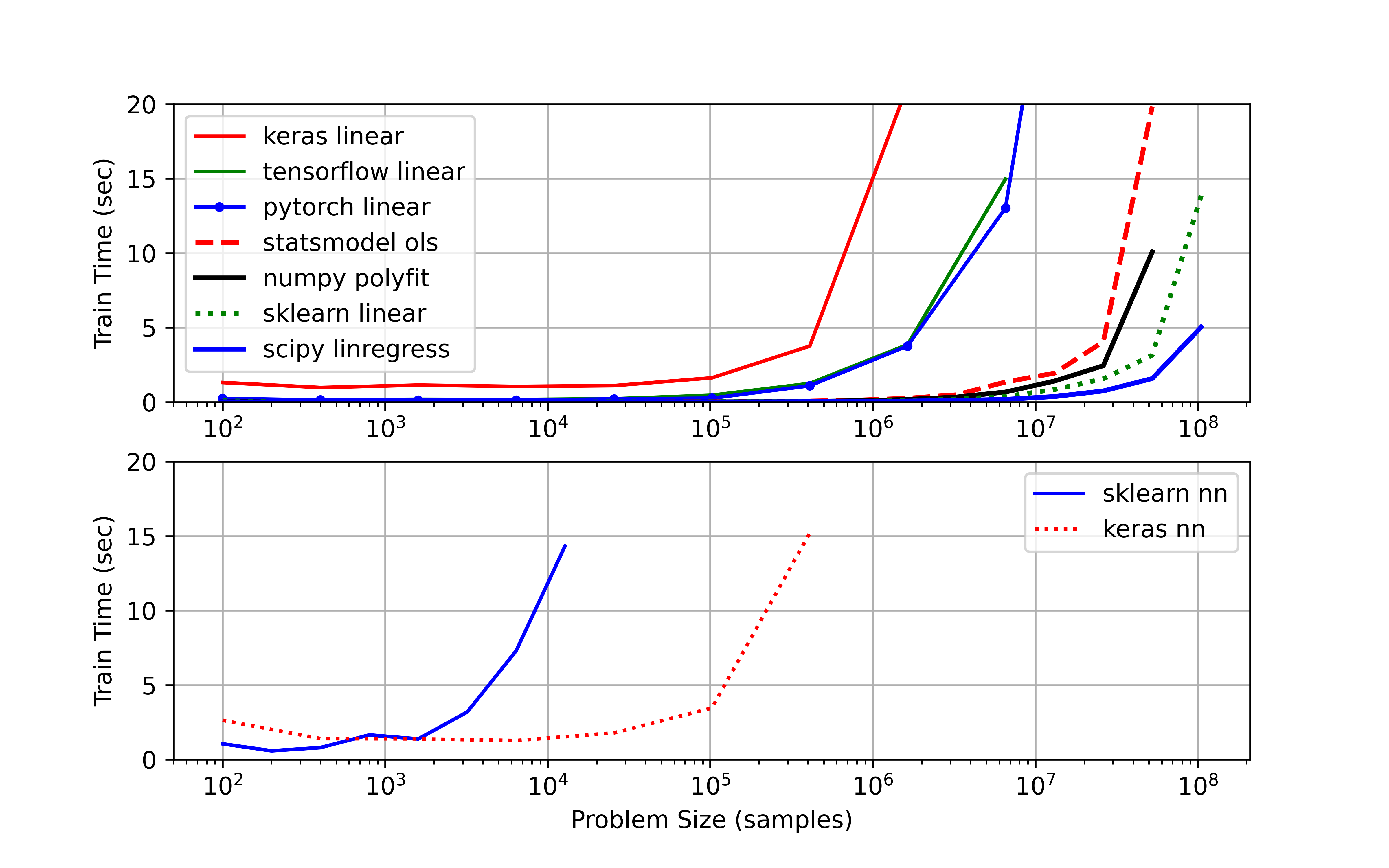
Linear Regression with GPU (Google Colab with GPU Kernel)
Changed test_time = 5.0 to avoid exceeding RAM limit for upgrading to Colab Pro subscription.
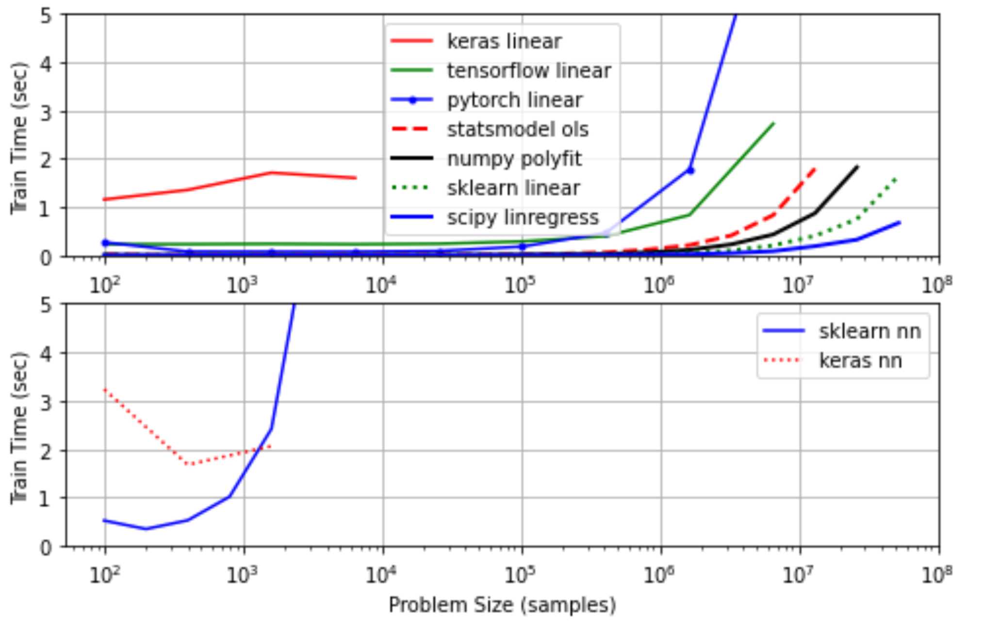
The results also include a bottom subplot that shows a neural network trained on the same data.
MATLAB Live Script

Given the content, here are two questions related to Linear Regression that expose common misconceptions:
✅ Knowledge Check
1. Which of the following statements best describes Linear Regression?
- Incorrect. Linear regression is used to predict continuous dependent variables.
- Incorrect. Linear regression assumes a linear relationship between the predictor and response variables.
- Correct. This is a common assumption in linear regression to ensure that the model is accurate and meaningful.
- Incorrect. The correct formula is `y = m \times x + c` where m is the slope and c is the intercept.
2. In multiple linear regression, how do the predictor variables relate to the response variable?
- Incorrect. In multiple linear regression, predictor variables contribute linearly to predict the response variable.
- Incorrect. Multiple linear regression uses more than one predictor variable.
- Incorrect. The relationship is represented using a single equation, but with multiple terms for each predictor.
- Correct. This is the essence of multiple linear regression.