Image Classification: Bits and Cracks

Objective: Train and test a Convolutional Neural Network to detect drilling bit types: roller cone, Polycrystalline Diamond Compact (PDC), and spoon types.
Deep Learning (DL) is a subset of Machine Learning that uses Neural Network inspired architecture to make predictions. Convolutional Neural Networks (CNN) are a type of DL model that is effective in learning patterns in 2-dimensional data such as images. Images of drill bit types are used to train a classifier to identify common drill bit types for Oil & Gas Exploration and Horizontal Directional Drilling (HDD).


This exercise demonstrates the use of image classification to distinguish between objects in photos. Although applied to bit types, the same methods and code can be used for any type or number of objects. This example can be modified by including train and test photos in folders that are named with the object type. The code automatically takes the name of the folder as the photo label for training the classifier. An additional example of an image-based CNN is found in the Soil Classification Case Study.
Getting Started
There are a few required packages for these exercises and can be installed with pip. These include OpenCV and TensorFlow from Google.
pip install tensorflow
This exercise uses photos of drill bit types in a compressed archive.
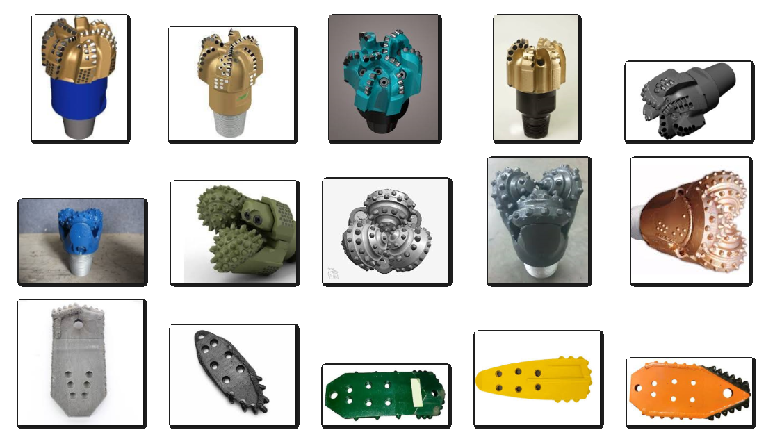
The archive contains two folders, a test folder and train folder with subdirectories corresponding to the possible drill bit types (PDC, Roller Cone, and Spoon). The images are found within each subdirectory. The tree structure of the folders is:
  ├───test
  │   ├───PDC
  │   ├───Roller Cone
  │   └───Spoon
  └───train
      ├───PDC
      ├───Roller Cone
      └───Spoon
The photos are imported into the Python session. The first step is to process the images into a format that 1) makes the data readable to the model, and 2) provides more training material for the model to learn. For example, the train_processor variable scales the data so that it can be a feature (input) for the model, but also takes each images and augments it so that the model can learn from multiple variations of the same picture. It flips it horizontally, rotates it, and shifts it, and more to make sure the model learns from the shape of the bit rather than the orientation or size.
import zipfile
import urllib.request
import cv2
import re
import random
import numpy as np
import matplotlib.pyplot as plt
from tensorflow.keras.preprocessing import image
from tensorflow.keras.preprocessing.image import ImageDataGenerator
from tensorflow.keras.models import Sequential
from tensorflow.keras.layers import Dense, Activation, Flatten
from tensorflow.keras.layers import Conv2D, MaxPooling2D
# download bit_photos.zip
file = 'bit_photos.zip'
url = 'http://apmonitor.com/pds/uploads/Main/'+file
urllib.request.urlretrieve(url, file)
# extract archive and remove bit_photos.zip
with zipfile.ZipFile(file, 'r') as zip_ref:
zip_ref.extractall('./')
os.remove(file)
# Data processing
train_processor = ImageDataGenerator(rescale = 1./255, \
horizontal_flip = True, zoom_range = 0.2, \
rotation_range = 10, shear_range = 0.2, \
height_shift_range = 0.1, width_shift_range = 0.1)
test_processor = ImageDataGenerator(rescale = 1./255)
# Load data
train = train_processor.flow_from_directory('train', \
target_size = (256, 256), batch_size = 32, \
class_mode = 'categorical', shuffle = True)
test = test_processor.flow_from_directory('test', \
target_size = (256 ,256), batch_size = 32, \
class_mode = 'categorical', shuffle = False)
# choose model parameters
num_conv_layers = 2
num_dense_layers = 1
layer_size = 64
num_training_epochs = 20
model = Sequential()
# begin adding properties to model variable
# e.g. add a convolutional layer
model.add(Conv2D(layer_size, (3, 3), input_shape=(256,256, 3)))
model.add(Activation('relu'))
model.add(MaxPooling2D(pool_size=(2, 2)))
# add additional convolutional layers based on num_conv_layers
for _ in range(num_conv_layers-1):
model.add(Conv2D(layer_size, (3, 3)))
model.add(Activation('relu'))
model.add(MaxPooling2D(pool_size=(2, 2)))
# reduce dimensionality
model.add(Flatten())
# add fully connected "dense" layers if specified
for _ in range(num_dense_layers):
model.add(Dense(layer_size))
model.add(Activation('relu'))
# add output layer
model.add(Dense(3))
model.add(Activation('softmax'))
# compile the sequential model with all added properties
model.compile(loss='categorical_crossentropy',
optimizer='adam',
metrics=['accuracy'],
)
# use the data already loaded previously to train/tune the model
model.fit(train,
epochs=num_training_epochs,
validation_data = test)
# save the trained model
model.save(f'bits.h5')
btype = ['PDC', 'Roller Cone', 'Spoon'] # possible output values
def make_prediction(image_fp):
im = cv2.imread(image_fp) # load image
plt.imshow(im)
img = image.load_img(image_fp, target_size = (256,256))
img = image.img_to_array(img)
image_array = img / 255. # scale the image
img_batch = np.expand_dims(image_array, axis = 0)
predicted_value = btype[model.predict(img_batch).argmax()]
true_value = re.search(r'(PDC)|(Roller Cone)|(Spoon)', image_fp)[0]
out = f"""Predicted Bit Type: {predicted_value}
True Bit Type: {true_value}
Correct?: {predicted_value == true_value}"""
return out
# randomly select type (1-3) and image number (1-5)
i = random.randint(0,2); j = random.randint(1,5)
b = btype[i]; im = b.replace(' ','_').lower() + '_' + str(j) + '.jpg'
test_image_filepath = r'./test/'+b+'/'+im
print(make_prediction(test_image_filepath))
plt.show()
The next step is to build the Convolutional Neural Network (CNN) model. Options are number of convolutional layers, fully connected dense layers, the number of nodes in each layer, and the number of training epochs. For more information on these parameters and CNNs in general, see Computer Vision with Deep Learning.
The model has now been trained and has been saved as an h5 file. The last line of the printed output contains the accuracy for both the training and testing data.
  Epoch 19/20
    accuracy: 0.6202 - val_loss: 0.9091 - val_accuracy: 0.6000
  Epoch 20/20
    accuracy: 0.5721 - val_loss: 0.8648 - val_accuracy: 0.6667
The val_accuracy is the accuracy on the test images (not included in the training). Hyperparameter optimization can be used to improve the accuracy by adjusting the CNN architecture, training selections, or other parameters. The function make_prediction takes the file path to a drill bit photo as an input and produces a classification result.
The validation accuracy as well as individual testing shows that there are misclassifications. Here are a few things that can improve the accuracy for this application:
- More photos! This is the most important thing, Machine Learning typically requires many photos that are representative of what the classifiers see. At this point, there are not nearly enough photos for the model to learn each bit type.
- Background Clutter Most of the images in this set have the background removed. To train a classifier to identify bit types in the field, more photos with realistic backgrounds are needed. Synthetic backgrounds can also be added.
- Hyperparameter Optimization To make the best model, the best parameters must be selected to maximize the accuracy (hyperparameter optimization). Packages such as Hyperopt try different parameter combinations to increase the accuracy.
Exercise
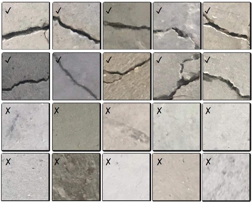
Replace the photos in the bit classification case study to build a classifier to distinguish photos of concrete with a crack (Positive) or no crack (Negative).
The images are found within each subdirectory. The tree structure of the folders is:
  ├───test
  │   ├───Positive
  │   └───Negative
  └───train
      ├───Positive
      └───Negative
The dataset is divided into two (negative and positive) crack image folders for image classification. Each train folder has 500 images with a total of 1000 images with 227 x 227 pixels with RGB channels. The test folders have 100 images from the full image set for a total of 200 test images. The partial dataset trains much faster and gives similar accuracy (95%) versus 97% for the full data set with 40,000 images.
Solutions

import zipfile
import urllib.request
import numpy as np
import matplotlib.pyplot as plt
from tensorflow.keras.preprocessing import image
from tensorflow.keras.preprocessing.image import ImageDataGenerator
from tensorflow.keras.models import Sequential
from tensorflow.keras.layers import Dense, Activation, Flatten
from tensorflow.keras.layers import Conv2D, MaxPooling2D
# download concrete_cracks.zip
file = 'concrete_cracks.zip'
url = 'http://apmonitor.com/pds/uploads/Main/'+file
urllib.request.urlretrieve(url, file)
# extract archive and remove concrete_cracks.zip
with zipfile.ZipFile(file, 'r') as zip_ref:
zip_ref.extractall('./')
os.remove(file)
# Data processing
train_processor = ImageDataGenerator(rescale = 1./255, \
horizontal_flip = True, zoom_range = 0.2, \
rotation_range = 10, shear_range = 0.2, \
height_shift_range = 0.1, width_shift_range = 0.1)
test_processor = ImageDataGenerator(rescale = 1./255)
# Load data
train = train_processor.flow_from_directory('train', \
target_size = (128,128), batch_size = 32, \
class_mode = 'categorical', shuffle = True)
test = test_processor.flow_from_directory('test', \
target_size = (128,128), batch_size = 32, \
class_mode = 'categorical', shuffle = False)
# choose model parameters
num_conv_layers = 2
num_dense_layers = 1
layer_size = 16
num_training_epochs = 5
model = Sequential()
# begin adding properties to model variable
# e.g. add a convolutional layer
model.add(Conv2D(layer_size, (3, 3), input_shape=(128,128,3)))
model.add(Activation('relu'))
model.add(MaxPooling2D(pool_size=(2, 2)))
# add additional convolutional layers based on num_conv_layers
for _ in range(num_conv_layers-1):
model.add(Conv2D(layer_size, (3, 3)))
model.add(Activation('relu'))
model.add(MaxPooling2D(pool_size=(2, 2)))
# reduce dimensionality
model.add(Flatten())
# add fully connected "dense" layers if specified
for _ in range(num_dense_layers):
model.add(Dense(layer_size))
model.add(Activation('relu'))
# add output layer
model.add(Dense(2))
model.add(Activation('softmax'))
# compile the sequential model with all added properties
model.compile(loss='categorical_crossentropy',
optimizer='adam',
metrics=['accuracy'],
)
# use the data already loaded previously to train/tune the model
model.fit(train,
epochs=num_training_epochs,
validation_data = test)
# save the trained model
model.save(f'cracks.h5')
 Download cracks.h5 TensorFlow Model to Skip Training
import re
import random
import numpy as np
import matplotlib.pyplot as plt
from tensorflow.keras.preprocessing import image
from tensorflow.keras.preprocessing.image import ImageDataGenerator
from tensorflow import keras
# Data processing
test_processor = ImageDataGenerator(rescale = 1./255)
test = test_processor.flow_from_directory('test', \
target_size = (128, 128), batch_size = 32, \
class_mode = 'categorical', shuffle = False)
# load the trained model
model = keras.models.load_model('cracks.h5')
ctype = ['Negative','Positive'] # possible output values
def make_prediction(image_fp):
im = cv2.imread(image_fp) # load image
plt.imshow(im)
img = image.load_img(image_fp, target_size = (128,128))
img = image.img_to_array(img)
image_array = img / 255. # scale the image
img_batch = np.expand_dims(image_array, axis = 0)
predicted_value = ctype[model.predict(img_batch).argmax()]
true_value = re.search(r'(Negative)|(Positive)', image_fp)[0]
out = f"""Predicted Crack: {predicted_value}
True Crack: {true_value}
Correct?: {predicted_value == true_value}"""
return out
# randomly select type (2) and image number (19901-20000)
i = random.randint(0,1); j = random.randint(19901,20000)
b = ctype[i]; im = str(j) + '.jpg'
test_image_filepath = r'./test/'+b+'/'+im
print(make_prediction(test_image_filepath))
plt.show()
References
- Özgenel, Ç.F., Gönenç Sorguç, A. “Performance Comparison of Pretrained Convolutional Neural Networks on Crack Detection in Buildings”, ISARC 2018, Berlin.
- Zhang, L., Yang, F., Zhang, Y.D., Zhu, Y.J., Road Crack Detection Using Deep Convolutional Neural Network. In 2016 IEEE International Conference on Image Processing (ICIP). DOI:10.1109/ICIP.2016.7533052, 2016.
Thanks to Peter Van Katwyk for generating the bit classification case study.

Solutions