Data Gathering and Consolidation
Gathering data is the process of consolidating disparate data (Excel spreadsheet, CSV file, PDF report, database, cloud storage) into a single repository. Data may reside in local storage or obtained through a remote connection to a database, web service, or extracted from a webpage.


Generate a data table dx and save it as a Comma Separated Values (CSV) file to be used as an example.
Generate Sample Data dx.csv
import pandas as pd
tx = np.linspace(0,1,8); x = np.cos(tx)
dx = pd.DataFrame({'Time':tx,'x':x})
dx.to_csv('dx.csv',index=False)
print(dx)

| Time | x |
| 0.000000 | 1.000000 |
| 0.142857 | 0.989813 |
| 0.285714 | 0.959461 |
| 0.428571 | 0.909560 |
| 0.571429 | 0.841129 |
| 0.714286 | 0.755561 |
| 0.857143 | 0.654600 |
| 1.000000 | 0.540302 |
Pandas

An easy way to read a data file is with Pandas. It produces a DataFrame that is a table with headers. The data source can either be local
pd.read_csv('dx.csv')
or from an online source such as a URL.
pd.read_csv('http://apmonitor.com/pds/uploads/Main/dx.txt')
Pandas can also read tables from a webpage such as the data table from this page.
table = pd.read_html(url)
print(table)
   [          0         1
    0      Time         x
    1  0.000000  1.000000
    2  0.142857  0.989813
    3  0.285714  0.959461
    4  0.428571  0.909560
    5  0.571429  0.841129
    6  0.714286  0.755561
    7  0.857143  0.654600
    8  1.000000  0.540302]
If there is more than one table on a page then Pandas reads each one as a list of DataFrames. There are additional read options in Pandas such as from the Clipboard, Excel, Feather, Flat file, Google BigQuery, HTML, JSON, HDFStore, Pickled Files, Parquet, ORC, SAS, SPSS, SQL Database, and STATA. There are also options to write a DataFrame to a CSV file or to the following data structures or online repositories.
dx.to_clipboard()
dx.to_csv()
dx.to_dict()
dx.to_excel()
dx.to_feather()
dx.to_gbq()
dx.to_hdf()
dx.to_html()
dx.to_json()
dx.to_latex()
dx.to_markdown()
dx.to_parquet()
dx.to_pickle()
dx.to_records()
dx.to_sql()
dx.to_stata()
dx.to_string()
Numpy

There are Numpy functions for loading data files. The function genfromtxt replaces any non-numeric values (such as a header) with nan (not a number).
print(d)
   [[       nan        nan]
    [0.         1.        ]
    [0.14285714 0.98981326]
    [0.28571429 0.95946058]
    [0.42857143 0.90956035]
    [0.57142857 0.84112921]
    [0.71428571 0.75556135]
    [0.85714286 0.65460007]
    [1.         0.54030231]]
The function loadtxt skips a certain number of rows that may contain non-numeric values.
print(d)
   [[0.         1.        ]
    [0.14285714 0.98981326]
    [0.28571429 0.95946058]
    [0.42857143 0.90956035]
    [0.57142857 0.84112921]
    [0.71428571 0.75556135]
    [0.85714286 0.65460007]
    [1.         0.54030231]]
Numpy functions are fast but limited to only numeric data that can fit into a standard Numpy data structure such as an array.
Open and Read File
Sometimes more control is needed to process complex data files. The open() function returns a file object f. This script opens the file dx.csv, prints each line, and closes the file.
for x in f:
print(x)
f.close()
   Time,x
   0.0,1.0
   0.14285714285714285,0.9898132604466151
   0.2857142857142857,0.9594605811119173
   0.42857142857142855,0.9095603516741667
   0.5714285714285714,0.8411292134152362
   0.7142857142857142,0.7555613467006966
   0.8571428571428571,0.6546000666752676
   1.0,0.5403023058681398
The read() function returns the contents of the entire file. A number such as read(4) returns only the first 4 characters.
x = f.read(4); print(x)
f.close()
Time
The readline() function returns the next line of the file.
print(f.readline())
print(f.readline())
print(f.readline())
f.close()
   Time,x
   0.0,1.0
   0.14285714285714285,0.9898132604466151
Beautiful Soup

Beautiful Soup is a Python package for extracting (scraping) information from web pages. It uses an HTML or XML parser and functions for iterating, searching, and modifying the parse tree.
First, get the html source from a webpage such as this page.
url = 'http://apmonitor.com/pds/index.php/Main/GatherData?action=print'
page = requests.get(url)
The attribute page.content contains the html source if page_status_code starts with a 2 such as 200 (downloaded successfully). A 4 or 5 indicates an error. BeautifulSoup parses HTML or XML files.
soup = BeautifulSoup(page.content, 'html.parser')
Functions such as print(soup.prettify()) can be used to view the structured output or the page title
Data Gathering and Consolidation
All of the links are extracted:
print('Link Text: {}'.format(link.text))
print('href: {}'.format(link.get('href')))
   Link Text: Data Gathering and Consolidation
   href: https://apmonitor.com/pds/index.php/Main/GatherData
   Link Text: Data File
   href: https://apmonitor.com/pds/uploads/Main/dx.txt
Pandas uses BeautifulSoup to extract tables from webpages. Data scraping is particularly useful for getting information from webpages that are updated with new information such as weather, stock data, and customer reviews. More advanced web scraping packages are Scrapy and Selenium.
Join Data
For time series data, the tables are joined to match features and labels at particular time points.
Generate DataFrames dx and dy
import pandas as pd
tx = np.linspace(0,1,4); x = np.cos(tx)
dx = pd.DataFrame({'Time':tx,'x':x})
ty = np.linspace(0,1,3); y = np.sin(ty)
dy = pd.DataFrame({'Time':ty,'y':y})
          Time         x
   0  0.000000  1.000000
   1  0.333333  0.944957
   2  0.666667  0.785887
   3  1.000000  0.540302

          Time         y
   0       0.0  0.000000
   1       0.5  0.479426
   2       1.0  0.841471
The two dataframes are joined with an index ('Time') that is set as the key for comparing and merging.
dy = dy.set_index('Time')
Options for merging are to join only the entries of dy that match dx.
All missing entries have NaN for Not a Number. The default is a left join meaning that DataFrame z has the same index as x.
                    x         y
   Time
   0.000000  1.000000  0.000000
   0.333333  0.944957       NaN
   0.666667  0.785887       NaN
   1.000000  0.540302  0.841471
Right Join
A right join results in the index of y.
                x         y
   Time
   0.0   1.000000  0.000000
   0.5        NaN  0.479426
   1.0   0.540302  0.841471
Inner Join
An inner join gives only the rows with an index that is common to both DataFrames.
                x         y
   Time
   0.0   1.000000  0.000000
   1.0   0.540302  0.841471
Outer Join
An outer join with sort=True gives all of the entries from both DataFrames.
                    x         y
   Time
   0.000000  1.000000  0.000000
   0.333333  0.944957       NaN
   0.500000       NaN  0.479426
   0.666667  0.785887       NaN
   1.000000  0.540302  0.841471
Append Data
Multiple data sets can be combined with the .append() function. This is needed to combine multiple data sets with the same types of data but stored separately.
import pandas as pd
tx = np.linspace(0,1,4); x = np.cos(tx)
dx = pd.DataFrame({'Time':tx,'x':x})
tx = np.linspace(0,1,3)
x = np.cos(tx)
dy = pd.DataFrame({'Time':tx,'x':x})
In this case, both dx and dy have the same data but at different times.
          Time         x
   0  0.000000  1.000000
   1  0.333333  0.944957
   2  0.666667  0.785887
   3  1.000000  0.540302

          Time         x
       0   0.0  1.000000
       1   0.5  0.877583
       2   1.0  0.540302
The functions append, sort_values, drop_duplicates, and reset_index are used to append, sort, consolidate, and reset the index of the table.
.sort_values(by='Time')\
.drop_duplicates(subset='Time')\
.reset_index(drop=True)
          Time         x
   0  0.000000  1.000000
   1  0.333333  0.944957
   2  0.500000  0.877583
   3  0.666667  0.785887
   4  1.000000  0.540302
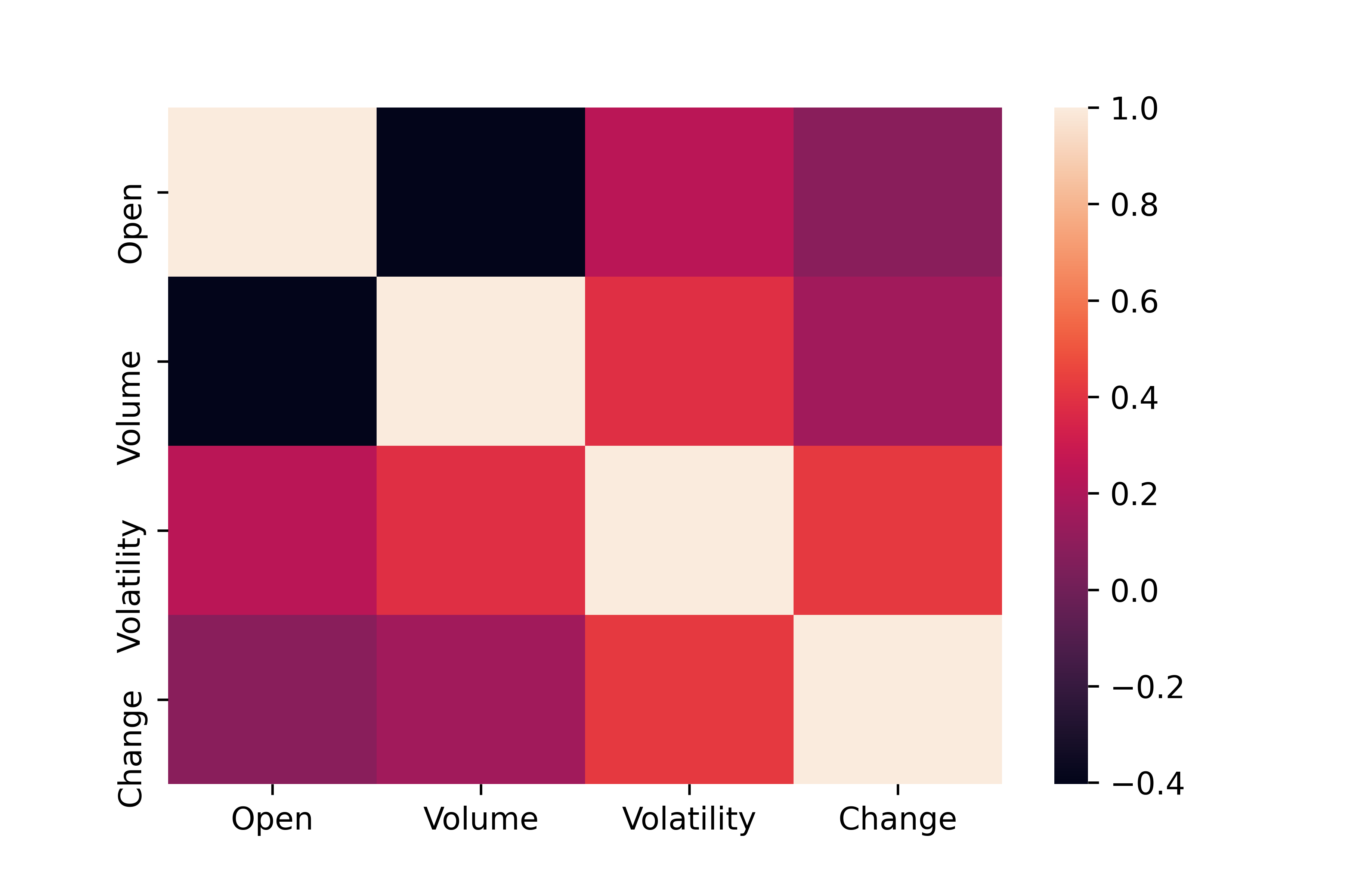
Activity

Import Google Stock Data and display the table.
Calculate summary statistics such as the mean, median, standard deviation, and quartile information. Create two new data columns for Volatility=High-Low and Change=Close-Open.
Solution
import matplotlib.pyplot as plt
import seaborn as sns
# stock ticker symbol
url = 'http://apmonitor.com/pds/uploads/Main/goog.txt'
# import data with pandas
data = pd.read_csv(url)
print(data.describe())
# calculate change and volatility
data['Change'] = data['Close']-data['Open']
data['Volatility'] = data['High']-data['Low']
analysis = ['Open','Volume','Volatility','Change']
sns.heatmap(data[analysis].corr())
plt.show()
✅ Knowledge Assessment
1. Which of the following best describes the process of data gathering?
- Incorrect. Data gathering involves actively collecting data, not just storing it.
- Incorrect. While it's essential to manage redundant data, data gathering itself focuses on the collection and consolidation of data.
- Correct. Data gathering involves actively collecting data from different sources for analysis or decision-making.
- Incorrect. Analysis is a subsequent step after data gathering. Data gathering focuses on the collection process.
2. What does data consolidation involve?
- Incorrect. Data consolidation is about bringing data together, not creating multiple copies of it.
- Correct. Data consolidation means combining data from various sources to present it in a unified manner or view.
- Incorrect. Data consolidation implies the intention to use combined data, not merely collecting without a purpose.
- Incorrect. While analysis may follow consolidation, the consolidation itself is about combining data.