Classification with Machine Learning


Classification is the problem of identifying which set of categories based on observation features. The decision is based on a training set of data containing observations where category membership is known (supervised learning) or where category membership is unknown (unsupervised learning).

A basic example is to determine the number from pixelated images in a built-in sklearn dataset. The script predicts 0-9 from the following images with a Support Vector Classifier.
classifier = svm.SVC(gamma=0.001)
# Learn / Fit
classifier.fit(X_train, y_train)
# Predict
classifier.predict(digits.data[n:n+1])[0]
from sklearn.model_selection import train_test_split
from sklearn.metrics import confusion_matrix, ConfusionMatrixDisplay
import matplotlib.pyplot as plt
import numpy as np
# The digits dataset
digits = datasets.load_digits()
n_samples = len(digits.images)
data = digits.images.reshape((n_samples, -1))
# Create support vector classifier
classifier = svm.SVC(gamma=0.001)
# Split into train and test subsets (50% each)
X_train, X_test, y_train, y_test = train_test_split(
data, digits.target, test_size=0.5, shuffle=False)
# Learn the digits on the first half of the digits
classifier.fit(X_train, y_train)
# test on second half of data
n = np.random.randint(int(n_samples/2),n_samples)
plt.imshow(digits.images[n], cmap=plt.cm.gray_r, interpolation='nearest')
print('Predicted: ' + str(classifier.predict(digits.data[n:n+1])[0]))
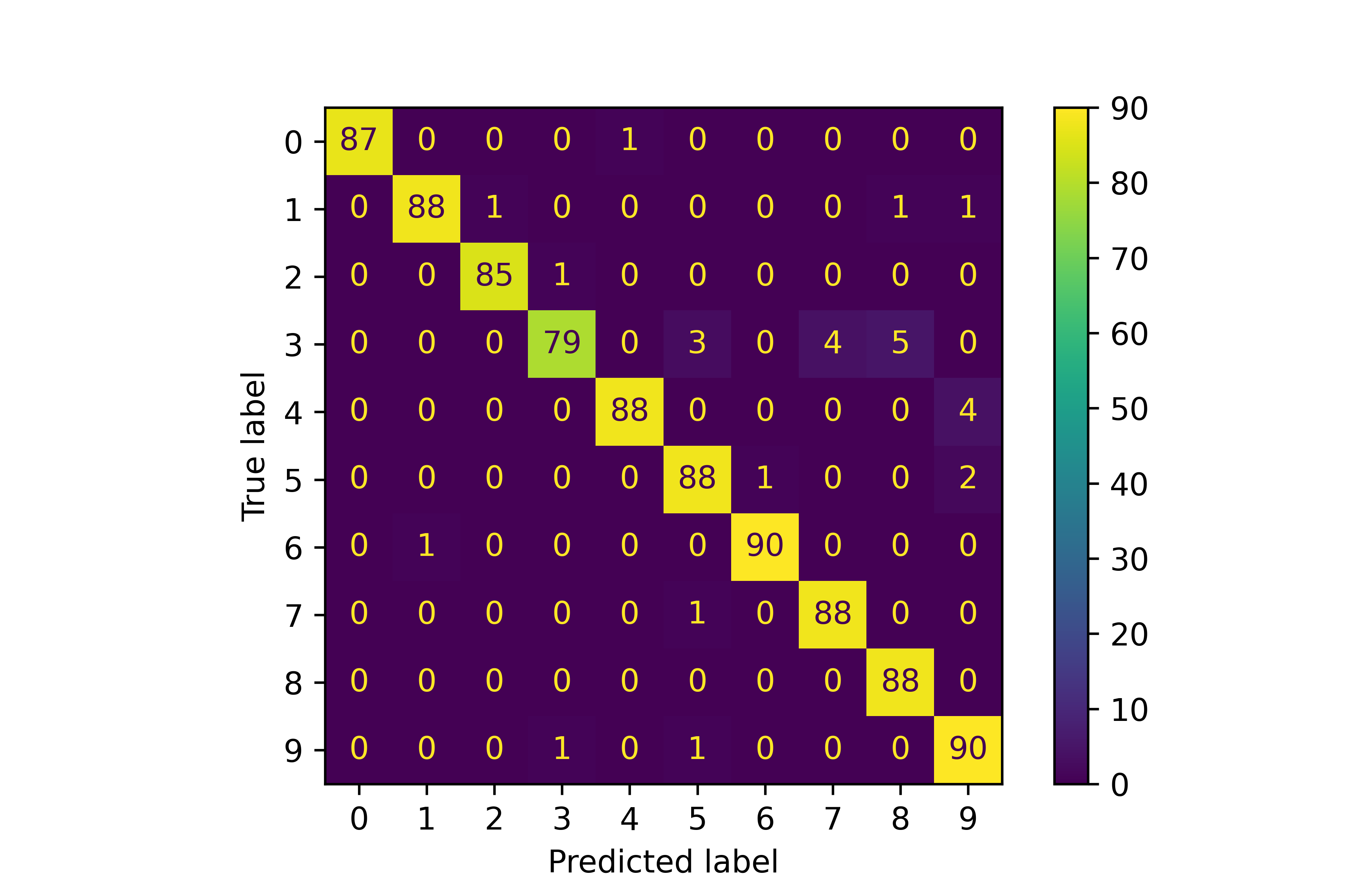
# generate confusion matrix
disp = metrics.plot_confusion_matrix(classifier, X_test, y_test)
# Get the predictions from the classifier
predictions = classifier.predict(X_test)
# Compute the confusion matrix
cm = confusion_matrix(y_test, predictions)
# Plot the confusion matrix
disp = ConfusionMatrixDisplay(confusion_matrix=cm)
disp.plot()
The confusion matrix shows the number of digits that are correctly classified and how the digits that are misclassified.
A convolutional neural network (simple CNN) shows how a number is classified with each layer.
from sklearn.model_selection import train_test_split
import matplotlib.pyplot as plt
import numpy as np
import time
# The digits dataset
digits = datasets.load_digits()
n_samples = len(digits.images)
data = digits.images.reshape((n_samples, -1))
# Split into train and test subsets (50% each)
XA, XB, yA, yB = train_test_split(
data, digits.target, test_size=0.5, shuffle=False)
# Logistic Regression
from sklearn.linear_model import LogisticRegression
lr = LogisticRegression(solver='lbfgs',multi_class='auto',max_iter=2000)
# Naïve Bayes
from sklearn.naive_bayes import GaussianNB
nb = GaussianNB()
# Stochastic Gradient Descent
from sklearn.linear_model import SGDClassifier
sgd = SGDClassifier(loss='modified_huber', shuffle=True,random_state=101,\
tol=1e-3,max_iter=1000)
# K-Nearest Neighbors
from sklearn.neighbors import KNeighborsClassifier
knn = KNeighborsClassifier(n_neighbors=10)
# Decision Tree
from sklearn.tree import DecisionTreeClassifier
dtree = DecisionTreeClassifier(max_depth=10,random_state=101,\
max_features=None,min_samples_leaf=5)
# Random Forest
from sklearn.ensemble import RandomForestClassifier
rfm = RandomForestClassifier(n_estimators=70,oob_score=True,n_jobs=1,\
random_state=101,max_features=None,min_samples_leaf=3)
# Support Vector Classifier
from sklearn.svm import SVC
svm = SVC(gamma='scale', C=1.0, random_state=101)
# Neural Network
from sklearn.neural_network import MLPClassifier
nn = MLPClassifier(solver='lbfgs',alpha=1e-5,max_iter=200,\
activation='relu',hidden_layer_sizes=(10,30,10),\
random_state=1, shuffle=True)
# classification methods
m = [nb,lr,sgd,knn,dtree,rfm,svm,nn]
s = ['nb','lr','sgd','knn','dt','rfm','svm','nn']
# fit classifiers
print('Train Classifiers')
for i,x in enumerate(m):
st = time.time()
x.fit(XA,yA)
tf = str(round(time.time()-st,5))
print(s[i] + ' time: ' + tf)
# test on random number in second half of data
n = np.random.randint(int(n_samples/2),n_samples)
Xt = digits.data[n:n+1]
# test classifiers
print('Test Classifiers')
for i,x in enumerate(m):
st = time.time()
yt = x.predict(Xt)
tf = str(round(time.time()-st,5))
print(s[i] + ' predicts: ' + str(yt[0]) + ' time: ' + tf)
print('Label: ' + str(digits.target[n:n+1][0]))
plt.imshow(digits.images[n], cmap=plt.cm.gray_r, interpolation='nearest')
plt.show()
from sklearn.datasets import load_digits
from sklearn.model_selection import train_test_split
data = load_digits()
X = data.data
y = data.target
# train / test split
X_train, X_test, y_train, y_test = train_test_split(X, y,
test_size=.5,random_state=12)
# exclude classifiers
clf_select = []
exclude = ['LGBMClassifier', 'DummyClassifier']
for x in CLASSIFIERS:
if not any(x[0] == ex for ex in exclude):
clf_select.append(x[1])
# fit classifiers
clf = LazyClassifier(verbose=0,ignore_warnings=True, \
custom_metric=None,classifiers=clf_select)
models,predictions = clf.fit(X_train, X_test, y_train, y_test)
print(models)
models.to_csv('models.csv')
| Model | Accuracy | Bal Acc | F1 Score | Time |
| SVC | 0.98 | 0.98 | 0.98 | 0.11 |
| ExtraTreesClassifier | 0.97 | 0.97 | 0.97 | 0.21 |
| RandomForestClassifier | 0.97 | 0.97 | 0.97 | 0.28 |
| LGBMClassifier | 0.97 | 0.97 | 0.97 | 0.67 |
| KNeighborsClassifier | 0.96 | 0.96 | 0.96 | 0.07 |
| LogisticRegression | 0.96 | 0.96 | 0.96 | 0.06 |
| XGBClassifier | 0.96 | 0.96 | 0.96 | 0.28 |
| CalibratedClassifierCV | 0.95 | 0.95 | 0.95 | 0.59 |
| LinearDiscriminantAnalysis | 0.95 | 0.95 | 0.95 | 0.04 |
| SGDClassifier | 0.95 | 0.95 | 0.95 | 0.03 |
| LinearSVC | 0.95 | 0.95 | 0.95 | 0.12 |
| LabelSpreading | 0.95 | 0.95 | 0.95 | 0.15 |
| LabelPropagation | 0.95 | 0.95 | 0.95 | 0.13 |
| NuSVC | 0.94 | 0.94 | 0.94 | 0.18 |
| PassiveAggressiveClassifier | 0.93 | 0.93 | 0.93 | 0.04 |
| Perceptron | 0.93 | 0.93 | 0.93 | 0.02 |
| BaggingClassifier | 0.93 | 0.93 | 0.93 | 0.09 |
| RidgeClassifierCV | 0.92 | 0.92 | 0.92 | 0.03 |
| RidgeClassifier | 0.92 | 0.92 | 0.92 | 0.02 |
| QuadraticDiscriminantAnalysis | 0.88 | 0.88 | 0.88 | 0.02 |
| NearestCentroid | 0.88 | 0.88 | 0.88 | 0.05 |
| BernoulliNB | 0.87 | 0.87 | 0.87 | 0.01 |
| DecisionTreeClassifier | 0.82 | 0.82 | 0.82 | 0.02 |
| GaussianNB | 0.79 | 0.78 | 0.79 | 0.01 |
| ExtraTreeClassifier | 0.71 | 0.71 | 0.72 | 0.01 |
| AdaBoostClassifier | 0.27 | 0.28 | 0.2 | 0.16 |
| DummyClassifier | 0.1 | 0.1 | 0.02 | 0.01 |
In this case, the 8x8 (64) pixels are the input features to the classifier. The output of the classifier is a number from 0 to 9. The classifier is trained on 898 images and tested on the other 50% of the data. This is an example of supervised learning where the data is labeled with the correct number. An unsupervised learning method would not have the number labels on the training set. An unsupervised learning method creates categories instead of using labels.
The first step in classification is to curate the data. This typically involves enumeratation, scaling, outlier detection, and splitting the data into training, test, and an optional validation set. One way to learn about classification methods is through concrete examples where the results are visualized as 2D data. The homogeneous data needs data labels (True/False) because there is no segregation of the data that is required for unsupervised learning methods.
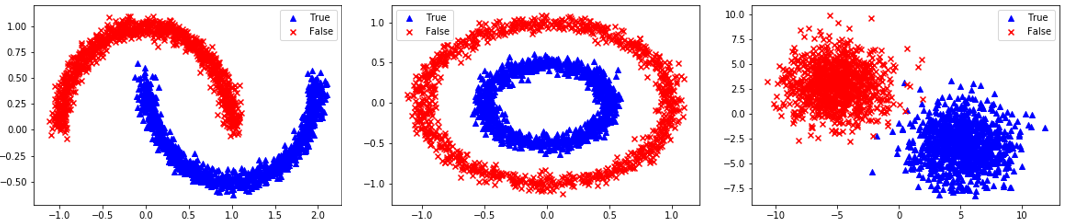
Homogeneous Population: 0=Linear, 1=Quadratic, 2=Target
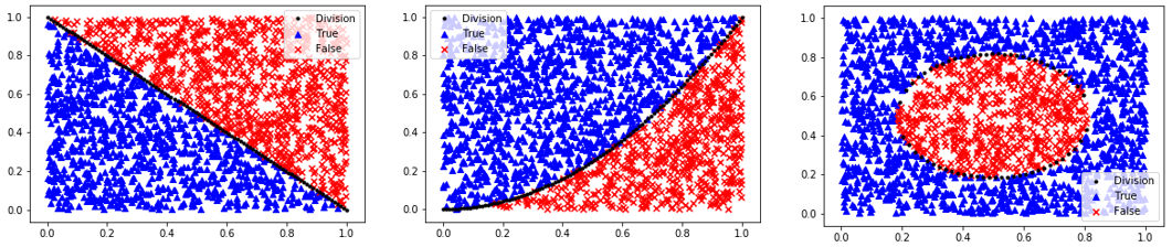
Segregated Clusters: 3=Moons, 4=Concentric Circles, 5=Distinct Clusters
data_options = ['linear','quadratic','target','moons','circles','blobs']
option = data_options[select_option]
n = 2000 # number of data points
X = np.random.random((n,2))
mixing = 0.0 # add random mixing element to data
xplot = np.linspace(0,1,100)
if option=='linear':
y = np.array([False if (X[i,0]+X[i,1])>=(1.0+mixing/2-np.random.rand()*mixing) \
else True \
for i in range(n)])
yplot = 1-xplot
elif option=='quadratic':
y = np.array([False if X[i,0]**2>=X[i,1]+(np.random.rand()-0.5)*mixing \
else True \
for i in range(n)])
yplot = xplot**2
elif option=='target':
y = np.array([False if (X[i,0]-0.5)**2+(X[i,1]-0.5)**2<=0.1 +(np.random.rand()-0.5)*0.2*mixing \
else True \
for i in range(n)])
j = False
yplot = np.empty(100)
for i,x in enumerate(xplot):
r = 0.1-(x-0.5)**2
if r<=0:
yplot[i] = np.nan
else:
j = not j # plot both sides of circle
yplot[i] = (2*j-1)*np.sqrt(r)+0.5
elif option=='moons':
X, y = datasets.make_moons(n_samples=n,noise=0.05)
yplot = xplot*0.0
elif option=='circles':
X, y = datasets.make_circles(n_samples=n,noise=0.05,factor=0.5)
yplot = xplot*0.0
elif option=='blobs':
X, y = datasets.make_blobs(n_samples=n,centers=[[-5,3],[5,-3]],cluster_std=2.0)
yplot = xplot*0.0
plt.scatter(X[y>0.5,0],X[y>0.5,1],color='blue',marker='^',label='True')
plt.scatter(X[y<0.5,0],X[y<0.5,1],color='red',marker='x',label='False')
if option not in ['moons','circles','blobs']:
plt.plot(xplot,yplot,'k.',label='Division')
plt.legend()
# Split into train and test subsets (50% each)
XA, XB, yA, yB = train_test_split(X, y, test_size=0.5, shuffle=False)
# Plot regression results
def assess(P):
plt.figure()
plt.scatter(XB[P==1,0],XB[P==1,1],marker='^',color='blue',label='True')
plt.scatter(XB[P==0,0],XB[P==0,1],marker='x',color='red',label='False')
plt.scatter(XB[P!=yB,0],XB[P!=yB,1],marker='s',color='orange',alpha=0.5,label='Incorrect')
if option not in ['moons','circles','blobs']:
plt.plot(xplot,yplot,'k.',label='Division')
plt.legend()
For each of the supervised and unsupervised machine learning methods, the strengths and weaknesses are detailed. The more popular methods are reviewed although there are many new methods that are developed each year. The same principles of training, testing, and deployment are common to most learning methods.

Classification with Supervised Learning
- AdaBoost (Adaptive Boosting)
- Logistic Regression
- Naïve Bayes
- Stochastic Gradient Descent
- K-Nearest Neighbors
- Decision Tree
- Random Forest
- Support Vector Classifier
- Deep Learning Neural Network
- XGBoost Classifier
Classification with Unsupervised Learning
Summary
Classification with machine learning is through supervised (labeled outcomes), unsupervised (unlabeled outcomes), or with semi-supervised (some labeled outcomes) methods. From the many methods for classification the best one depends on the problem objectives, data characteristics, and data availability. Below is a complete compilation of the source code for supervised and unsupervised learning methods. Scikit-learn documentation has a comparison of other supervised learning methods.
from sklearn.model_selection import train_test_split
import matplotlib.pyplot as plt
import numpy as np
# The digits dataset
digits = datasets.load_digits()
# Flatten the image to apply classifier
n_samples = len(digits.images)
data = digits.images.reshape((n_samples, -1))
# Create support vector classifier
classifier = svm.SVC(gamma=0.001)
# Split into train and test subsets (50% each)
X_train, X_test, y_train, y_test = train_test_split(
data, digits.target, test_size=0.5, shuffle=False)
# Learn the digits on the first half of the digits
classifier.fit(X_train, y_train)
n_samples/2
# test on second half of data
n = np.random.randint(int(n_samples/2),n_samples)
plt.imshow(digits.images[n], cmap=plt.cm.gray_r, interpolation='nearest')
print('Predicted: ' + str(classifier.predict(digits.data[n:n+1])[0]))
# Select Option by Number
# 0 = Linear, 1 = Quadratic, 2 = Inner Target
# 3 = Moons, 4 = Concentric Circles, 5 = Distinct Clusters
select_option = 5
# generate data
data_options = ['linear','quadratic','target','moons','circles','blobs']
option = data_options[select_option]
# number of data points
n = 2000
X = np.random.random((n,2))
mixing = 0.0 # add random mixing element to data
xplot = np.linspace(0,1,100)
if option=='linear':
y = np.array([False if (X[i,0]+X[i,1])>=(1.0+mixing/2-np.random.rand()*mixing) else True for i in range(n)])
yplot = 1-xplot
elif option=='quadratic':
y = np.array([False if X[i,0]**2>=X[i,1]+(np.random.rand()-0.5)\
*mixing else True for i in range(n)])
yplot = xplot**2
elif option=='target':
y = np.array([False if (X[i,0]-0.5)**2+(X[i,1]-0.5)**2<=0.1 +(np.random.rand()-0.5)*0.2*mixing else True for i in range(n)])
j = False
yplot = np.empty(100)
for i,x in enumerate(xplot):
r = 0.1-(x-0.5)**2
if r<=0:
yplot[i] = np.nan
else:
j = not j # plot both sides of circle
yplot[i] = (2*j-1)*np.sqrt(r)+0.5
elif option=='moons':
X, y = datasets.make_moons(n_samples=n,noise=0.05)
yplot = xplot*0.0
elif option=='circles':
X, y = datasets.make_circles(n_samples=n,noise=0.05,factor=0.5)
yplot = xplot*0.0
elif option=='blobs':
X, y = datasets.make_blobs(n_samples=n,centers=[[-5,3],[5,-3]],cluster_std=2.0)
yplot = xplot*0.0
plt.scatter(X[y>0.5,0],X[y>0.5,1],color='blue',marker='^',label='True')
plt.scatter(X[y<0.5,0],X[y<0.5,1],color='red',marker='x',label='False')
if option not in ['moons','circles','blobs']:
plt.plot(xplot,yplot,'k.',label='Division')
plt.legend()
plt.savefig(str(select_option)+'.png')
# Split into train and test subsets (50% each)
XA, XB, yA, yB = train_test_split(X, y, test_size=0.5, shuffle=False)
# Plot regression results
def assess(P):
plt.figure()
plt.scatter(XB[P==1,0],XB[P==1,1],marker='^',color='blue',label='True')
plt.scatter(XB[P==0,0],XB[P==0,1],marker='x',color='red',label='False')
plt.scatter(XB[P!=yB,0],XB[P!=yB,1],marker='s',color='orange',alpha=0.5,label='Incorrect')
if option not in ['moons','circles','blobs']:
plt.plot(xplot,yplot,'k.',label='Division')
plt.legend()
# Supervised Classification
# Logistic Regression
from sklearn.linear_model import LogisticRegression
lr = LogisticRegression(solver='lbfgs')
lr.fit(XA,yA)
yP = lr.predict(XB)
assess(yP)
# Naïve Bayes
from sklearn.naive_bayes import GaussianNB
nb = GaussianNB()
nb.fit(XA,yA)
yP = nb.predict(XB)
assess(yP)
# Stochastic Gradient Descent
from sklearn.linear_model import SGDClassifier
sgd = SGDClassifier(loss='modified_huber', shuffle=True,random_state=101)
sgd.fit(XA,yA)
yP = sgd.predict(XB)
assess(yP)
# K-Nearest Neighbors
from sklearn.neighbors import KNeighborsClassifier
knn = KNeighborsClassifier(n_neighbors=5)
knn.fit(XA,yA)
yP = knn.predict(XB)
assess(yP)
# Decision Tree
from sklearn.tree import DecisionTreeClassifier
dtree = DecisionTreeClassifier(max_depth=10,random_state=101,max_features=None,\
min_samples_leaf=5)
dtree.fit(XA,yA)
yP = dtree.predict(XB)
assess(yP)
# Random Forest
from sklearn.ensemble import RandomForestClassifier
rfm = RandomForestClassifier(n_estimators=70,oob_score=True,n_jobs=1,\
random_state=101,max_features=None,min_samples_leaf=3)
rfm.fit(XA,yA)
yP = rfm.predict(XB)
assess(yP)
# Support Vector Classifier
from sklearn.svm import SVC
svm = SVC(gamma='scale', C=1.0, random_state=101)
svm.fit(XA,yA)
yP = svm.predict(XB)
assess(yP)
# Neural Network
from sklearn.neural_network import MLPClassifier
clf = MLPClassifier(solver='lbfgs',alpha=1e-5,max_iter=200,\
activation='relu',hidden_layer_sizes=(10,30,10),\
random_state=1, shuffle=True)
clf.fit(XA,yA)
yP = clf.predict(XB)
assess(yP)
# Unsupervised Classification
# K-Means Clustering
try:
from sklearn.cluster import KMeans
km = KMeans(n_clusters=2)
km.fit(XA)
yP = km.predict(XB)
# Arbitrary labels with unsupervised clustering
# may need to be reversed
if len(XB[yP!=yB]) > n/4: yP = 1 - yP
assess(yP)
except:
print('K-Means failed')
# Gaussian Mixture Model
from sklearn.mixture import GaussianMixture
gmm = GaussianMixture(n_components=2)
gmm.fit(XA)
yP = gmm.predict_proba(XB) # produces probabilities
# Arbitrary labels with unsupervised clustering may need to be reversed
if len(XB[np.round(yP[:,0])!=yB]) > n/4: yP = 1 - yP
assess(np.round(yP[:,0]))
# Spectral Clustering
from sklearn.cluster import SpectralClustering
sc = SpectralClustering(n_clusters=2,eigen_solver='arpack',\
affinity='nearest_neighbors')
yP = sc.fit_predict(XB) # No separation between fit and predict calls, need to fit and predict on same dataset
# Arbitrary labels with unsupervised clustering may need to be reversed
if len(XB[yP!=yB]) > n/4: yP = 1 - yP
assess(yP)
plt.show()