IOT/OT Cybersecurity
Operational Technology (OT) includes computer systems and equipment that make changes to the physical world. Sensors, actuators, and computer control systems are critical to safe operation and are increasingly under threat of attack. Industrial sectors include transportation, manufacturing, energy production, power generation, grid networks, and pipelines. A self-driving car has actuators such as steering direction, motor torque, and brake action. Airplane actuators include engine thrust, aileron angle, and flap position. Industrial chemical process actuators include valves and pumps. It is imperative that the commanded actuator is implemented as requested. There may be a difference between the commanded and actual state of the actuator if there is a cyberattack or equipment malfunction. Cyberattacks may be stealth changes to a process that go undetected but that cause equipment failure, lost economic potential, or HSE (Health, Safety, Environmental) incidents.


This is a case study with a microcontroller with sensors and actuators (TCLab) where the heater (actuator) is monitored to determine if it is on or off. The predicted and commanded heater states are compared to determine if there is an equipment failure or external actor that has taken control of the actuator. A TCLab digital twin is included if the hardware is not connected.
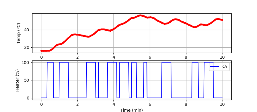
Develop a classifier to predict when the TCLab heater is on and when it is off. Generate labeled data where the heater is either on at 100% output or at 0% output for periods between 10 and 25 seconds.
Small Data Set (10 min)
The data set is split into a training and test set. The data is generated from a TCLab or sample data is accessed at the link below.

import numpy as np
import matplotlib.pyplot as plt
import pandas as pd
import tclab
import time
n = 600 # Number of second time points (10 min)
tm = np.linspace(0,n,n+1) # Time values
lab = tclab.TCLab()
T1 = [lab.T1]
T2 = [lab.T2]
Q1 = np.zeros(n+1)
Q2 = np.zeros(n+1)
# turn on heater at select times
Q1[20:41] = 100.0; Q1[60:91] = 100.0; Q1[150:181] = 100.0
Q1[190:206] = 100.0; Q1[220:251] = 100.0; Q1[260:291] = 100.0
Q1[300:316] = 100.0; Q1[340:351] = 100.0; Q1[400:431] = 100.0
Q1[500:521] = 100.0; Q1[540:571] = 100.0
for i in range(n):
lab.Q1(Q1[i]); lab.Q2(Q2[i])
time.sleep(1)
print(Q1[i],lab.T1)
T1.append(lab.T1); T2.append(lab.T2)
lab.close()
# Save data file
data = np.vstack((tm,Q1,Q2,T1,T2)).T
np.savetxt('tclab_test.csv',data,delimiter=',',\
header='Time,Q1,Q2,T1,T2',comments='')
# Create Figure
plt.figure(figsize=(10,7))
ax = plt.subplot(2,1,1)
ax.grid()
plt.plot(tm/60.0,T1,'r.',label=r'$T_1$')
plt.ylabel(r'Temp ($^oC$)')
ax = plt.subplot(2,1,2)
ax.grid()
plt.plot(tm/60.0,Q1,'b-',label=r'$Q_1$')
plt.ylabel(r'Heater (%)')
plt.xlabel('Time (min)')
plt.legend()
plt.savefig('tclab_test.png')
plt.show()
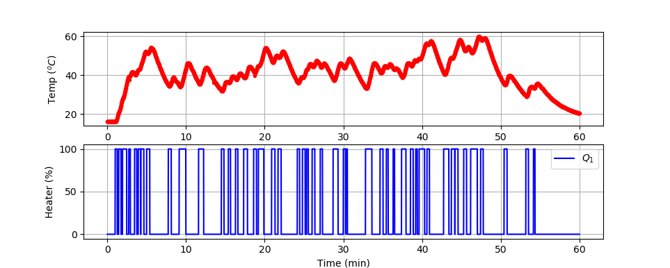
Large Data Set (1 hr)
import numpy as np
import matplotlib.pyplot as plt
import pandas as pd
import tclab
import time
n = 3600 # Number of second time points (60 min)
tm = np.linspace(0,n,n+1) # Time values
lab = tclab.TCLab()
T1 = [lab.T1]
T2 = [lab.T2]
Q1 = np.zeros(n+1)
Q2 = np.zeros(n+1)
# random duration on (10-30 sec) in 60 second window
# cool down last 5 minutes
k = 60
for i in range(1,n-301):
if (i%k)==0:
j = np.random.randint(10,26)
k = np.random.randint(5,180)
Q1[i:i+j+1] = 100.0
for i in range(n):
lab.Q1(Q1[i])
lab.Q2(Q2[i])
time.sleep(1)
print(Q1[i],lab.T1)
T1.append(lab.T1)
T2.append(lab.T2)
lab.close()
# Save data file
data = np.vstack((tm,Q1,Q2,T1,T2)).T
np.savetxt('tclab_train.csv',data,delimiter=',',\
header='Time,Q1,Q2,T1,T2',comments='')
# Create Figure
plt.figure(figsize=(10,7))
ax = plt.subplot(2,1,1)
ax.grid()
plt.plot(tm/60.0,T1,'r.',label=r'$T_1$')
plt.ylabel(r'Temp ($^oC$)')
ax = plt.subplot(2,1,2)
ax.grid()
plt.plot(tm/60.0,Q1,'b-',label=r'$Q_1$')
plt.ylabel(r'Heater (%)')
plt.xlabel('Time (min)')
plt.legend()
plt.savefig('tclab_train.png')
plt.show()
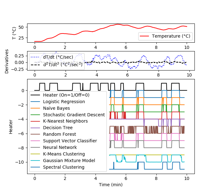
The features of the data are selected and scaled (0-1) such as temperature, and temperature derivatives. The measured temperature and derivatives and heater value labels are used to create a classifier that predicts when the heater is on or off. The classifier is validated with new data that was not used for training.
Classifier for 10 minute data set
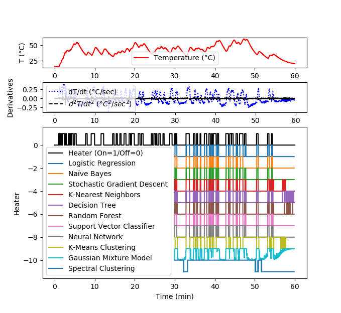
Classifier for 1 hour data set
import numpy as np
import matplotlib.pyplot as plt
from matplotlib import gridspec
from sklearn.preprocessing import MinMaxScaler
from sklearn.model_selection import train_test_split
# animate plot?
animate=False
# Load data
file1 = 'http://apmonitor.com/do/uploads/Main/tclab_data5.txt'
file2 = 'http://apmonitor.com/do/uploads/Main/tclab_data6.txt'
data = pd.read_csv(file2)
# Input Features: Temperature and 1st / 2nd Derivatives
# Cubic polynomial fit of temperature using 10 data points
data['dT1'] = np.zeros(len(data))
data['d2T1'] = np.zeros(len(data))
for i in range(len(data)):
if i<len(data)-10:
x = data['Time'][i:i+10]-data['Time'][i]
y = data['T1'][i:i+10]
p = np.polyfit(x,y,3)
# evaluate derivatives at mid-point (5 sec)
t = 5.0
data['dT1'][i] = 3.0*p[0]*t**2 + 2.0*p[1]*t+p[2]
data['d2T1'][i] = 6.0*p[0]*t + 2.0*p[1]
else:
data['dT1'][i] = np.nan
data['d2T1'][i] = np.nan
# Remove last 10 values
X = np.array(data[['T1','dT1','d2T1']][0:-10])
y = np.array(data[['Q1']][0:-10])
# Scale data
# Input features (Temperature and 2nd derivative at 5 sec)
s1 = MinMaxScaler(feature_range=(0,1))
Xs = s1.fit_transform(X)
# Output labels (heater On / Off)
ys = [True if y[i]>50.0 else False for i in range(len(y))]
# Split into train and test subsets (50% each)
XA, XB, yA, yB = train_test_split(Xs, ys, \
test_size=0.5, shuffle=False)
# Plot regression results
def assess(P):
plt.figure()
plt.scatter(XB[P==1,0],XB[P==1,1],marker='^',color='blue',label='True')
plt.scatter(XB[P==0,0],XB[P==0,1],marker='x',color='red',label='False')
plt.scatter(XB[P!=yB,0],XB[P!=yB,1],marker='s',color='orange',\
alpha=0.5,label='Incorrect')
plt.legend()
# Supervised Classification
# Logistic Regression
from sklearn.linear_model import LogisticRegression
lr = LogisticRegression(solver='lbfgs')
lr.fit(XA,yA)
yP1 = lr.predict(XB)
#assess(yP1)
# Naïve Bayes
from sklearn.naive_bayes import GaussianNB
nb = GaussianNB()
nb.fit(XA,yA)
yP2 = nb.predict(XB)
#assess(yP2)
# Stochastic Gradient Descent
from sklearn.linear_model import SGDClassifier
sgd = SGDClassifier(loss='modified_huber', shuffle=True,random_state=101)
sgd.fit(XA,yA)
yP3 = sgd.predict(XB)
#assess(yP3)
# K-Nearest Neighbors
from sklearn.neighbors import KNeighborsClassifier
knn = KNeighborsClassifier(n_neighbors=5)
knn.fit(XA,yA)
yP4 = knn.predict(XB)
#assess(yP4)
# Decision Tree
from sklearn.tree import DecisionTreeClassifier
dtree = DecisionTreeClassifier(max_depth=10,random_state=101,\
max_features=None,min_samples_leaf=5)
dtree.fit(XA,yA)
yP5 = dtree.predict(XB)
#assess(yP5)
# Random Forest
from sklearn.ensemble import RandomForestClassifier
rfm = RandomForestClassifier(n_estimators=70,oob_score=True,n_jobs=1,\
random_state=101,max_features=None,min_samples_leaf=3)
rfm.fit(XA,yA)
yP6 = rfm.predict(XB)
#assess(yP6)
# Support Vector Classifier
from sklearn.svm import SVC
svm = SVC(gamma='scale', C=1.0, random_state=101)
svm.fit(XA,yA)
yP7 = svm.predict(XB)
#assess(yP7)
# Neural Network
from sklearn.neural_network import MLPClassifier
clf = MLPClassifier(solver='lbfgs',alpha=1e-5,max_iter=200,\
activation='relu',hidden_layer_sizes=(10,30,10),\
random_state=1, shuffle=True)
clf.fit(XA,yA)
yP8 = clf.predict(XB)
#assess(yP8)
# Unsupervised Classification
# K-Means Clustering
from sklearn.cluster import KMeans
km = KMeans(n_clusters=2)
km.fit(XA)
yP9 = km.predict(XB)
# Arbitrary labels with unsupervised clustering may need to be reversed
#yP9 = 1.0-yP9
#assess(yP9)
# Gaussian Mixture Model
from sklearn.mixture import GaussianMixture
gmm = GaussianMixture(n_components=2)
gmm.fit(XA)
yP10 = gmm.predict_proba(XB) # produces probabilities
# Arbitrary labels with unsupervised clustering may need to be reversed
yP10 = 1.0-yP10[:,0]
# Spectral Clustering
from sklearn.cluster import SpectralClustering
sc = SpectralClustering(n_clusters=2,eigen_solver='arpack',\
affinity='nearest_neighbors')
yP11 = sc.fit_predict(XB) # No separation between fit and predict calls
# need to fit and predict on same dataset
# Arbitrary labels with unsupervised clustering may need to be reversed
#yP11 = 1.0-yP11
#assess(yP11)
plt.figure(figsize=(12,8))
if animate:
plt.ion()
plt.show()
make_gif = True
try:
import imageio # required to make gif animation
except:
print('install imageio with "pip install imageio" to make gif')
make_gif=False
if make_gif:
try:
import os
images = []
os.mkdir('./frames')
except:
print('Figure directory already created')
gs = gridspec.GridSpec(3, 1, height_ratios=[1,1,5])
plt.subplot(gs[0])
plt.plot(data['Time']/60,data['T1'],'r-',\
label='Temperature (°C)')
plt.ylabel('T (°C)')
plt.legend(loc=3)
plt.subplot(gs[1])
plt.plot(data['Time']/60,data['dT1'],'b:',\
label='dT/dt (°C/sec)')
plt.plot(data['Time']/60,data['d2T1'],'k--',\
label=r'$d^2T/dt^2$ ($°C^2/sec^2$)')
plt.ylabel('Derivatives')
plt.legend(loc=3)
plt.subplot(gs[2])
plt.plot(data['Time']/60,data['Q1']/100,'k-',\
label='Heater (On=1/Off=0)')
t2 = data['Time'][len(yA):-10].values
plt.plot(t2/60,yP1-1,label='Logistic Regression')
plt.plot(t2/60,yP2-2,label='Naïve Bayes')
plt.plot(t2/60,yP3-3,label='Stochastic Gradient Descent')
plt.plot(t2/60,yP4-4,label='K-Nearest Neighbors')
plt.plot(t2/60,yP5-5,label='Decision Tree')
plt.plot(t2/60,yP6-6,label='Random Forest')
plt.plot(t2/60,yP7-7,label='Support Vector Classifier')
plt.plot(t2/60,yP8-8,label='Neural Network')
plt.plot(t2/60,yP9-9,label='K-Means Clustering')
plt.plot(t2/60,yP10-10,label='Gaussian Mixture Model')
plt.plot(t2/60,yP11-11,label='Spectral Clustering')
plt.ylabel('Heater')
plt.xlabel(r'Time (min)')
plt.legend(loc=3)
if animate:
t = data['Time'].values/60
n = len(t)
for i in range(60,n+1,10):
for j in range(3):
plt.subplot(gs[j])
plt.xlim([t[max(0,i-1200)],t[i]])
filename='./frames/frame_'+str(1000+i)+'.png'
plt.savefig(filename)
if make_gif:
images.append(imageio.imread(filename))
plt.pause(0.1)
# create animated GIF
if make_gif:
imageio.mimsave('animate.gif', images)
imageio.mimsave('animate.mp4', images)
else:
plt.show()
Exercise
Simulate intermittent heater failure by turning down the heater power for periods of 30 seconds. The heater power is set with lab.P1. The heater power can be set from 0 to 255 and is set to 200 by default. The simulated cyber-attack turns off the heater by setting lab.P1=0 so that no energy is applied even though the heater is requested to a level of 100% on with lab.Q1(100).
import time
with tclab.TCLab() as lab:
# simulated cyber attack
print('Power Level (0-255): ' + str(lab.P1))
# test cyber attack
print('-'*40)
print('Heater Power Off')
print('Temperature (degC): ' + str(lab.T1))
lab.P1=0 # set heater 1 power level to zero
print('Power Level (0-255): ' + str(lab.P1))
lab.Q1(100) # turn on heater but no power (P1=0)
print('Wait 30 sec')
time.sleep(30)
print('Temperature (degC): ' + str(lab.T1))
print('-'*40)
print('Heater Power On')
print('Temperature (degC): ' + str(lab.T1))
lab.P1 = 200 # restore heater 1 power level
print('Power Level (0-255): ' + str(lab.P1))
lab.Q1(100) # turn on heater with power (P1=250)
print('Wait 30 sec')
time.sleep(30)
print('Temperature (degC): ' + str(lab.T1))
Use the classifier to detect when the heater has malfunctioned or is the target of a simulated cyberattack (the power is set to zero or the heater power supply is unplugged).

Solutions