Steel Plate Defects
Background: Steel plate defects are extracted from photos of several faulty steel plates with surface imperfections. Image analysis revealed 27 different features to describe the steel fault. A total of 6 unique types of faults are categorized, with a final category of "other faults" for any type of fault that does not fit into the other specific 6 categories.

url = 'http://apmonitor.com/pds/uploads/Main/steel.txt'
data = pd.read_csv(url)
Features: There are 27 features that are used to predict the steel faults. These features are extracted from steel plate samples. Computer vision can automatically extract some of this information from images or manually extracted with a user inspecting each plate defect or photo of the steel plate.
- X_Minimum
- X_Maximum
- Y_Minimum
- Y_Maximum
- Pixels_Areas
- X_Perimeter
- Y_Perimeter
- Sum_of_Luminosity
- Minimum_of_Luminosity
- Maximum_of_Luminosity
- Length_of_Conveyer
- TypeOfSteel_A300
- TypeOfSteel_A400
- Steel_Plate_Thickness
- Edges_Index
- Empty_Index
- Square_Index
- Outside_X_Index
- Edges_X_Index
- Edges_Y_Index
- Outside_Global_Index
- LogOfAreas
- Log_X_Index
- Log_Y_Index
- Orientation_Index
- Luminosity_Index
- SigmoidOfAreas
Labels: There are 7 types of steel plate defects that are labelled with a 1 if present and 0 if not present with One-Hot Encoding. A unique aspect of this data set is that the labels are imbalanced, meaning that there is a large difference in the number of specific defects.
- Pastry
- Z_Scratch
- K_Scatch
- Stains
- Dirtiness
- Bumps
- Other_Faults
In cases where there is a large imbalance, a strategy is to synthetically generate new data sets to improve the balance. That strategy is not taken in this case study but could be an option to improve the classification training. The fault label is not stored as a sequential value (e.g. fault label as 0-6) but is One-hot encoded to translate the fault label into a binary representation (0 or 1) for each fault. There are 7 additional columns of data with 1 if the fault exists and 0 if the fault does not exist.


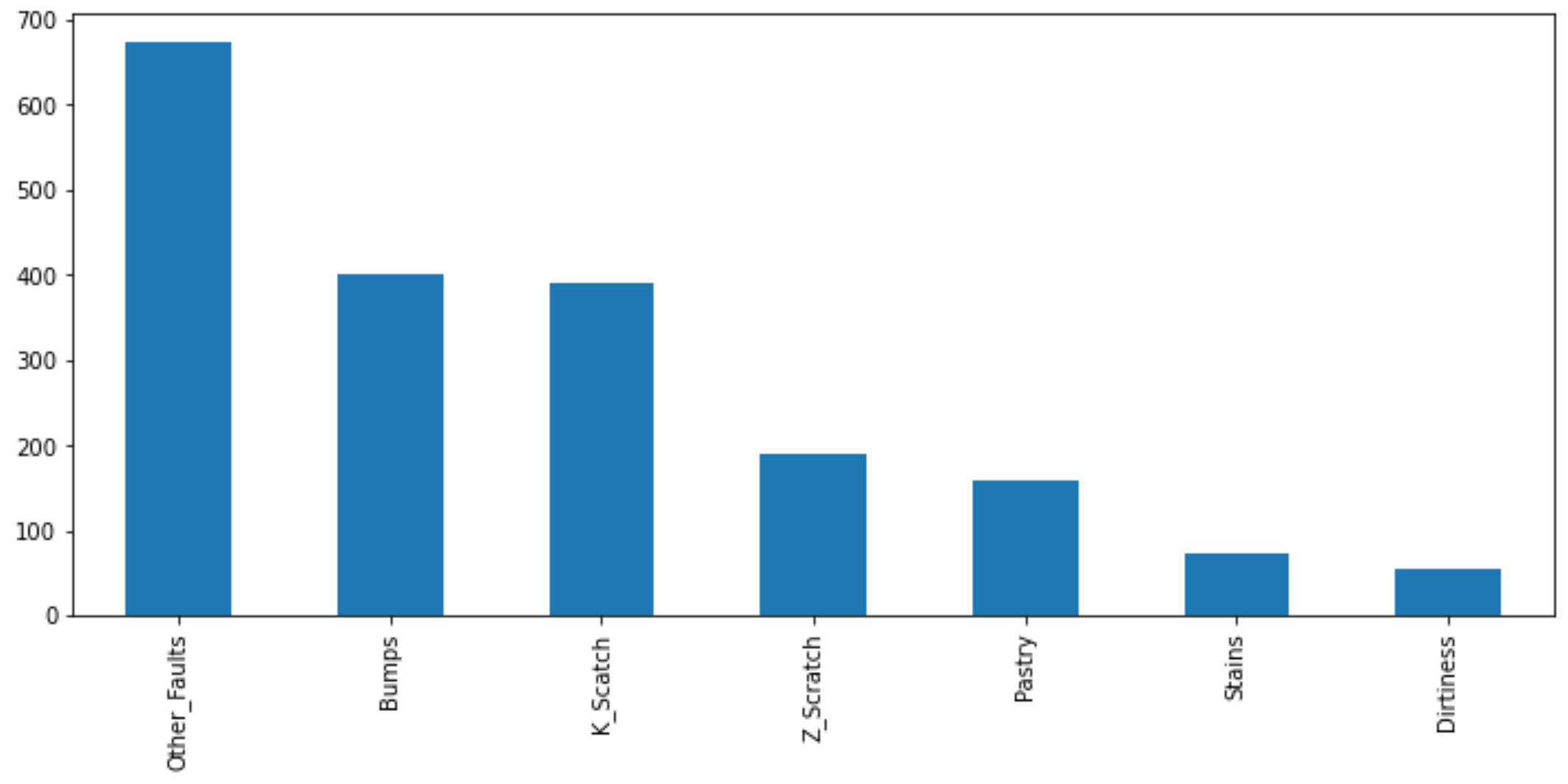
Data Exploration: Generate summary statistics with a profiling report to statistically characterize the data. Use box plots to identify any outliers in the data. Remove any outliers from the data set. Generate a pair plot and correlation matrix. What factors are highly correlated to the steel faults? Generate a bar chart that shows the imbalance of faults in the data.
features = data.columns[:-7]
labels = data.columns[-7:]
X = data[features]
y = data[labels]
y.idxmax(axis=1).value_counts().plot(kind='bar')
Classification of Faults: Train and test a classifier to distinguish between steel plate faults with Keras / TensorFlow.
from keras.models import Sequential
from keras.layers import Dense
# scikit-learn packages
from sklearn.metrics import confusion_matrix
from sklearn.preprocessing import MinMaxScaler
from sklearn.model_selection import train_test_split
from sklearn.feature_selection import SelectKBest,chi2
Randomly select values that split the data into a train (80%) and test (20%) set by using the scikit-learn function train_test_split
s = MinMaxScaler()
data_s = s.fit_transform(data)
data_s = pd.DataFrame(data_s,columns=data.columns)
# Split data into X and y
features = data.columns[:-7]
labels = data.columns[-7:]
X = data_s[features]
y = data_s[labels]
# Train/test split
Xtrain, Xtest, ytrain, ytest = train_test_split(X,y,test_size=0.2,shuffle=True)
or the keras validation_split=0.2 option.
model = Sequential()
model.add(Dense(8, input_dim=Xtrain.shape[1], activation='relu'))
model.add(Dense(ytrain.shape[1], activation='softmax'))
# Compile model
model.compile(loss='categorical_crossentropy', \
optimizer='adam', metrics=['accuracy'])
# Train model
result = model.fit(Xtrain,ytrain,epochs=1000,\
validation_split=0.2,verbose=0)
Determine any evidence of overfitting by plotting the training and test (validation) loss functions by epoch.
plt.semilogy(result.history['loss'],label='loss')
plt.semilogy(result.history['val_loss'],label='val_loss')
plt.legend()
plt.ylabel('Loss')
plt.xlabel('Epoch')
plt.show()
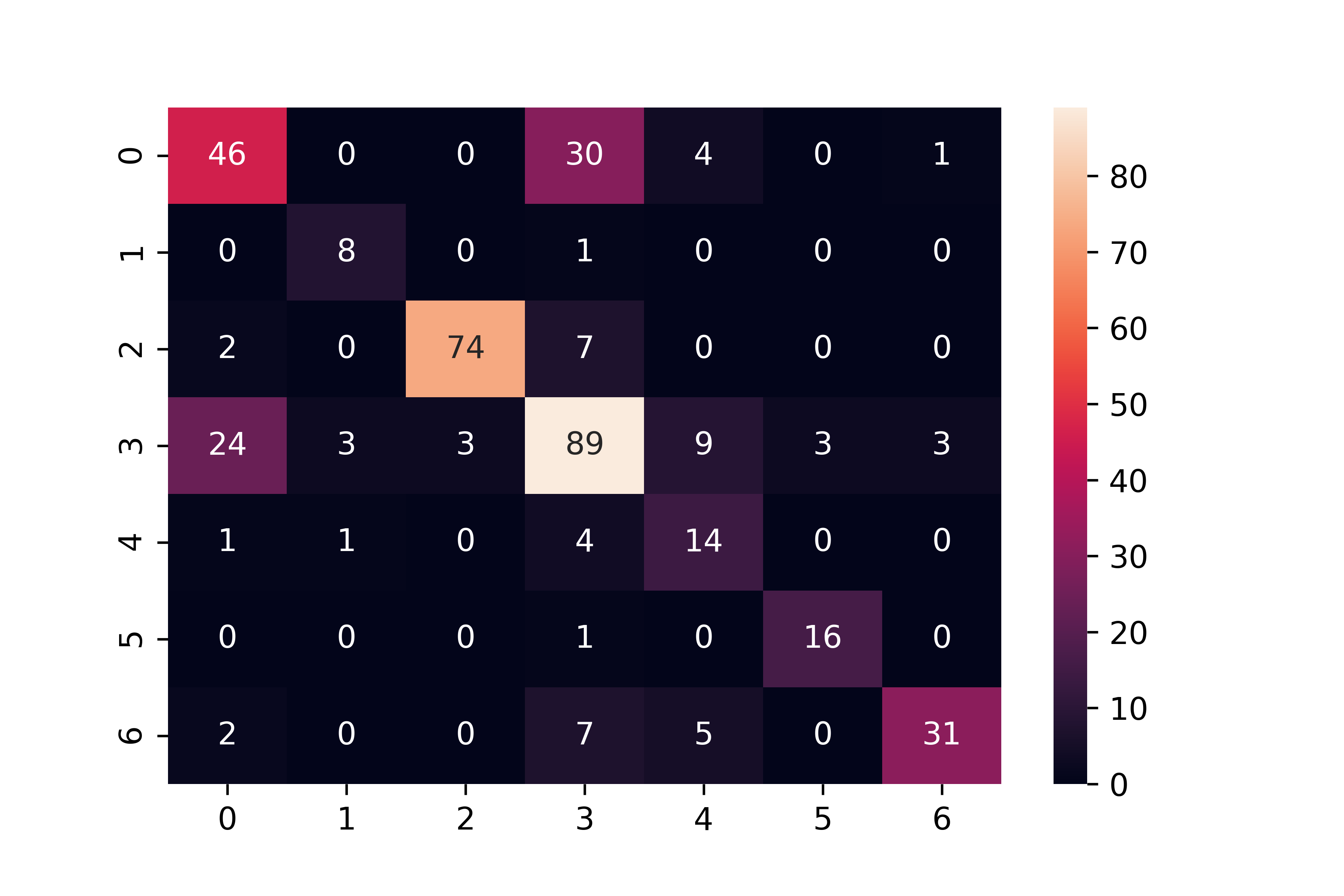
Confusion Matrix: Report the confusion matrix on the test set and discuss the performance. A confusion matrix shows correct classification (diagonal) and misclassification (off-diagonal).
yp = model.predict(Xtest)
yp = pd.DataFrame(yp,columns=ytest.columns)
# Extract predicted labels and probabilities
predicted_label = yp.idxmax(axis=1)
predicted_prob = yp.max(axis=1)
actual_label = ytest.idxmax(axis=1)
# highlighted and the actual label displayed
yp['Actual fault'] = actual_label.values
yp.style.highlight_max(axis=1)
# Plot the confusion matrix
cm = confusion_matrix(predicted_label,actual_label)
sns.heatmap(cm,annot=True)
plt.show()
Case Study Key Concepts
- Classification
- Imbalanced Labels
- Keras and TensorFlow Application
- Softmax Probabilities
References
- Dataset provided by Semeion, Research Center of Sciences of Communication, Via Sersale 117, 00128, Rome, Italy, URL: www.semeion.it UCI Data Set and Kaggle
- Fakhr, M., Elsayad, A.M., Steel Plates Faults Diagnosis with Data Mining Models, Journal of Computer Science 8 (4): 506-514, 2012. Article

Solutions