Machine Learning for Engineers

Imbalanced data is a disproportionate number of data points with discrete labels and can be a big challenge to develop an accurate classifier. A classifier attempts to find the data boundary where one class ends and the other begins. Classification is used to create these boundaries when the desired output (label) is discrete such as 0/1, Yes/No, 1,2,3,4,5, or Normal/Abnormal. Regression is used when the desired output (label) is continuous.

Imbalanced Data Python Jupyter Notebook

Jupyter Notebook in Google Colab

Imbalanced Data MATLAB Live Script

Imbalanced data can give biased predictions for classification when there is a minority class. This tutorial demonstrates how to deal with imbalanced data.

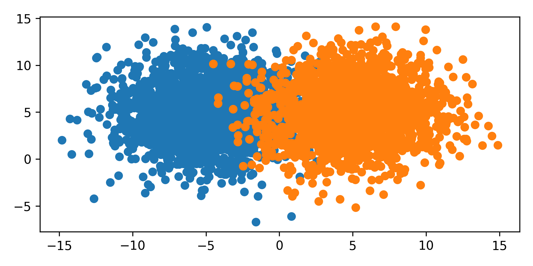
The dots are the color of the respective label. In this example, each class has the same size and spread and the the classifier splits the space in the middle. However, many data sets are imbalanced where every class is unequally sized, or weighted. This imbalance skews the classifier to favor the majority class.

from sklearn.datasets import make_blobs
from sklearn.linear_model import LogisticRegression
import numpy as np
import matplotlib.pyplot as plt

features, label = make_blobs(n_samples=[2000,50],\
                             n_features=2,\
                             centers=[(-5,5),(5,5)],\
                             random_state=47,cluster_std=3)
min1, max1 = features[:,0].min()-1,features[:,0].max()+1
min2, max2 = features[:,1].min()-1,features[:,1].max()+1

x1grid = np.arange(min1,max1,.1)
x2grid = np.arange(min2,max2,.1)

xx, yy = np.meshgrid(x1grid,x2grid)
r1,r2 = xx.flatten(), yy.flatten()
r1,r2 = r1.reshape((len(r1), 1)), r2.reshape((len(r2), 1))
grid = np.hstack((r1,r2))
model = LogisticRegression()
model.fit(features,label)

plt.figure(figsize=(6,3))
yp = model.predict(grid)
zz = yp.reshape(xx.shape)
plt.contourf(xx,yy,zz,cmap='Paired')
for cv in range(2):
    row = np.where(label==cv)
    plt.scatter(features[row,0],features[row,1],cmap = 'Paired')

plt.tight_layout()
plt.savefig('imbalanced_classification.png')
plt.show()

[$[Get Code]]

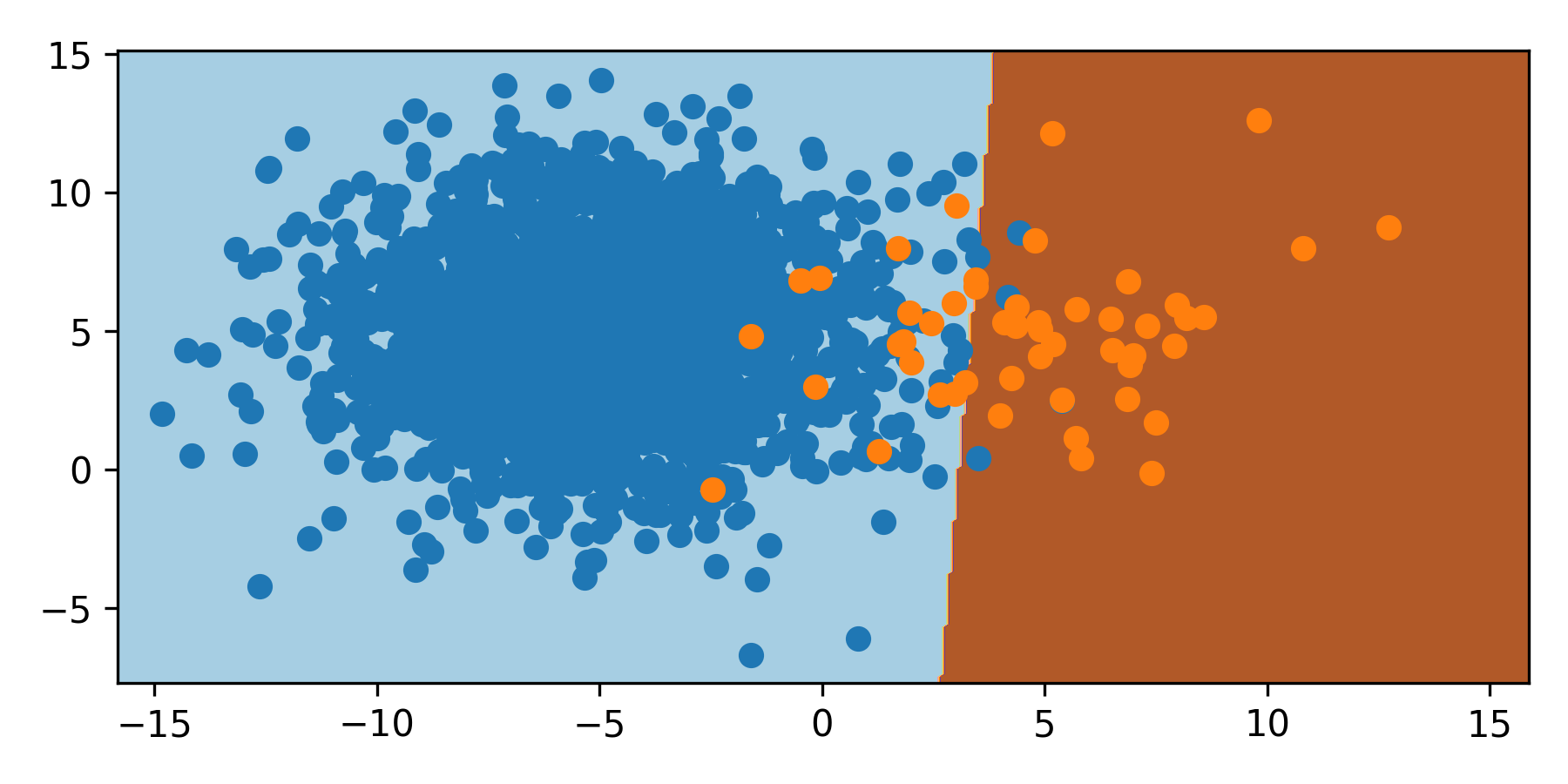
As the orange class has a smaller sampling, the classifier moves the boundary to the right. With 2000 samples of blue and 50 samples of orange, the boundary is shifted 3 units to the right and misclassifies the orange minority class.

Classification with Imbalanced Sets

There are multiple ways to deal with imbalanced datasets. Whenever possible, more samples should be obtained in the minority class or classes. When this is not possible, new data (oversampling the minority class) or data reduction (undersampling the majority class) are two ways to approach a balanced set. Install package imblearn to use the RandomUnderSampler and SMOTE.

Undersample Majority Class

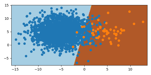
One way to deal with a much larger class is to undersample. This removes random instances from the majority class to reduce the number of instances to be comparable to the other classes. There are a few limitations to this. If the majority class is not sufficiently large, undersampling may lead to too little data overall for the model fit or validation. If the majority class samples are not normally distributed, stochastic undersampling can misshape the class, leading to additional errors. These factors should be considered before the decision to undersample. There is an improvement with undersampling the majority class in the synthetic data set.

Oversample Minority Class

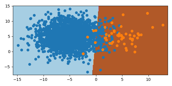
Oversampling is the opposite of undersampling. SMOTE (Synthetic Minority Oversampling TEchnique) is a method to oversample the minority class. SMOTE creates artificial sample points in the same area space as the minority class, allowing the model to weight the minority class and improve classifier accuracy. It must be noted, however, that these additional points are synthetic and if the minority class space is similar to that of another class, could lead to misclassification of other classes due to the expansion of the minority bounds in hyperspace.

Alternate Methods

Unsupervised learning methods such as K-means Clustering can train on the majority class and detect the minority class or classes as anomalies in the dataset. As an example, imagine a situation with four, similar-sized minority classes and one majority class where the majority class is much larger than the four minority classes. Anomaly detection, or binary classification, could be used to classify the data between “majority class” or “non-majority class”. A separate classifier could be trained on the “anomalous” data without the majority class. This subsequent model could then classify the data into any of the respective minority classes. This method can be chained and scaled to address imbalanced data.

Conclusion

Oversampling and undersampling both adjust the training data to more accurately classify the minority class.

Activity

The following imbalanced dataset has five features (inputs) and one label (output) with three classes (0,1,2).

Imbalanced Train Data

Imbalanced Test Data

The training set is undersampled from some true population, contained in the test set. Rebalance the training data to improve the classification of the minority class in the test set.

Imbalanced Notebook

Imbalanced Notebook (Solution)

Additional Reading

• Brownlee, J., SMOTE for Imbalanced Classification with Python, Imbalanced Classification, Machine Learning Mastery, Published January 17, 2020.
• Radečić, D., How to Effortlessly Handle Class Imbalance with Python and SMOTE, Towards Data Science, Published Dec 5, 2020.
• Goswami, S., SMOTE using Python: Achieving class balance with few lines of python codes, Towards Data Science, Published Feb 18, 2021.

✅ Knowledge Check

1. What does imbalanced data refer to?

2. Which of the following statements about imbalanced datasets is NOT true?