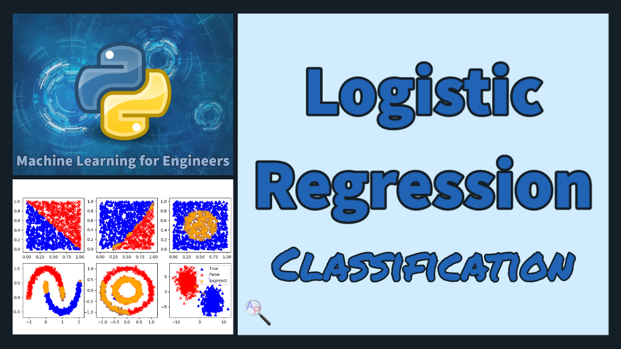
Logistic Regression
Logistic regression is a machine learning algorithm for classification. In this algorithm, the probabilities describing the possible outcomes of a single trial are modeled using a logistic function.


Logistic regression makes a binary classification prediction based on the sigmoid function with n input features, `x_1 \ldots x_n`.
$$p = \frac{1}{1+e^{-(\beta_0+\beta_1x_1+...+\beta_nx_n)}}$$
The `\beta_i` are coefficients that can be determined from a stochastic gradient descent or other optimization on the training dataset. The desired classification is either a 0 or 1, so the probability calculated with the sigmoid function is rounded to the nearest value.
Advantages: Logistic regression is designed for this purpose (classification), and is most useful for understanding the influence of several independent variables on a single outcome variable.
Disadvantages: Assumes all predictors are independent of each other, and assumes data set is free of missing values.
lr = LogisticRegression(solver='lbfgs')
lr.fit(XA,yA)
yP = lr.predict(XB)
Optical Character Recognition with Logistic Regression

Optical character recognition (OCR) is a method used to convert images of text into machine-readable text. It is typically used to process scanned documents and recognize the text in the images. Logistic regression is a type of machine learning model that can be used for classification tasks. In the context of OCR, logistic regression could be trained to recognize characters in images of text.
Here is an example of using logistic regression for OCR in Python:
from sklearn.datasets import load_digits
from sklearn.linear_model import LogisticRegression
from sklearn.model_selection import train_test_split
# Load the dataset of images of handwritten digits
digits = load_digits()
# Split the dataset into training and testing sets
X_train, X_test, y_train, y_test = train_test_split(digits.data,
digits.target,
random_state=0)
# Create a logistic regression classifier
clf = LogisticRegression(max_iter=5000, random_state=0)
# Train the model using the training set
clf.fit(X_train, y_train)
# Evaluate the model's performance on the test set
accuracy = clf.score(X_test, y_test)
print("Accuracy: %0.2f" % accuracy)
In this example, we use the scikit-learn library to load the dataset of images of handwritten digits, split the dataset into training and testing sets, and train a logistic regression classifier. We then evaluate the model's performance on the test set by computing the accuracy, which is the proportion of test images that the model correctly identifies. Below is an additional example that shows a sample image from the test set.
from sklearn.model_selection import train_test_split
import matplotlib.pyplot as plt
import numpy as np
from sklearn.linear_model import LogisticRegression
classifier = LogisticRegression(max_iter=5000,\
solver='lbfgs',\
multi_class='auto')
# The digits dataset
digits = datasets.load_digits()
n_samples = len(digits.images)
data = digits.images.reshape((n_samples, -1))
# Split into train and test subsets (50% each)
X_train, X_test, y_train, y_test = train_test_split(
data, digits.target, test_size=0.5, shuffle=False)
# Learn the digits on the first half of the digits
classifier.fit(X_train, y_train)
# Test on second half of data
n = np.random.randint(int(n_samples/2),n_samples)
print('Predicted: ' + str(classifier.predict(digits.data[n:n+1])[0]))
# Show number
plt.imshow(digits.images[n], cmap=plt.cm.gray_r, interpolation='nearest')
plt.show()

Logistic Regression Programming
Using only Python code (not a machine learning package), create a Logistic Regression classifier. Use the blobs test code to evaluate the performance of the code with any number of features (n_features). First develop the code to test 2 features. Use the source code blocks as needed.
import numpy as np
import matplotlib.pyplot as plt
from sklearn.datasets import make_blobs
import seaborn as sns
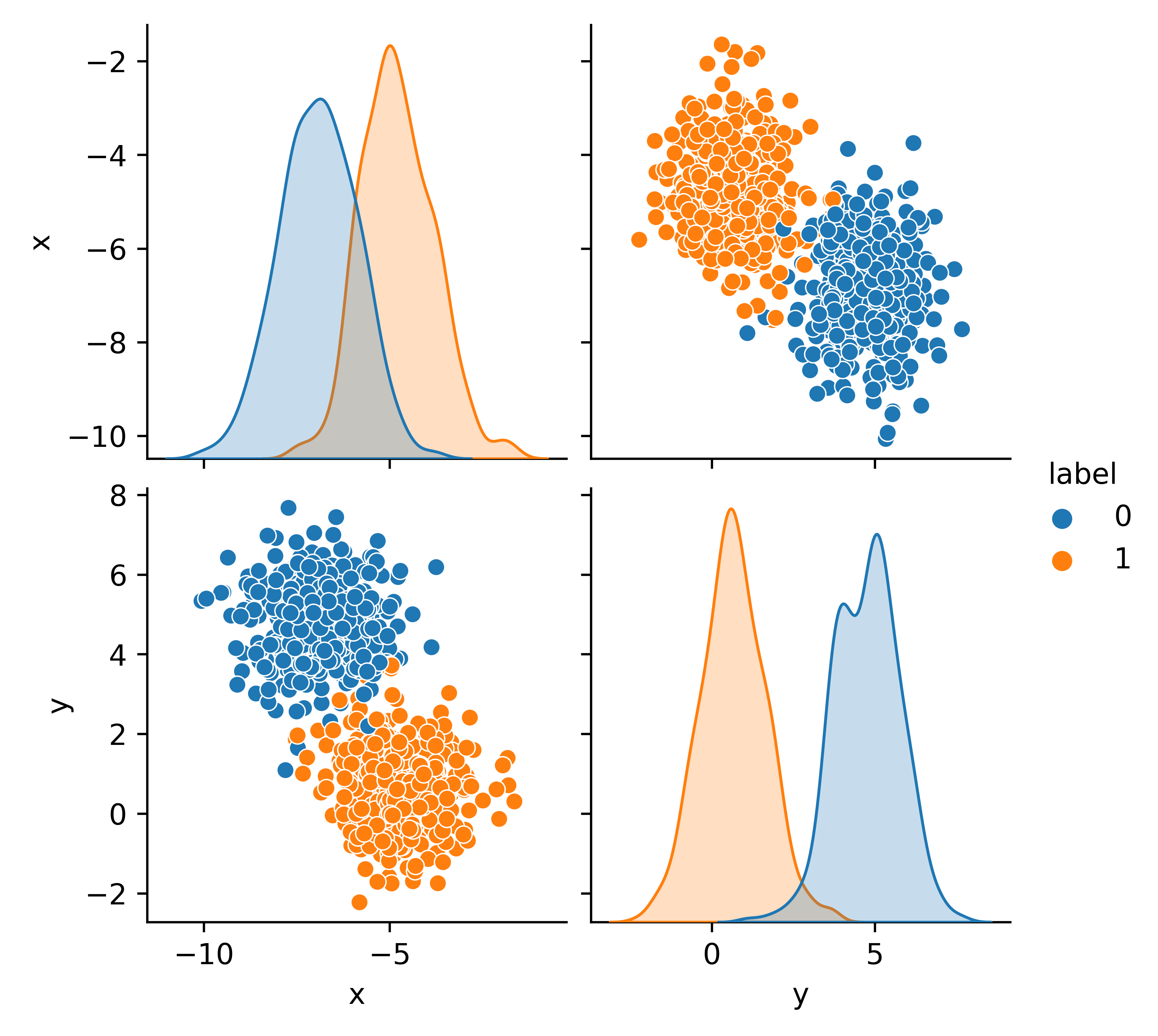
# Generate blobs dataset
features, label = make_blobs(n_samples=800, centers=2,\
n_features=2, random_state=12)
data = pd.DataFrame()
data['x1'] = features[:,0]
data['x2'] = features[:,1]
data['y'] = label
sns.pairplot(data,hue='y')
Split data into train (80%) and test (20%) sets.
train, test = train_test_split(data.values,test_size=0.2)
Create a function to make a prediction with coefficients.
$$p = \frac{1}{1+e^{-(\beta_0+\beta_1x_1+...+\beta_nx_n)}}$$
The predicted `\hat y` is `p` rounded to the nearest 0 or 1 to produce a final predicted value.
def predict(row, beta):
x = row[0:2]
t = beta[0] + beta[1]*x[0] + beta[2]*x[1]
return 1.0 / (1.0 + exp(-t))
Update coefficients for the intercept `\beta_0` with
$$\beta_0 = \beta_0 + l_{rate} (err) p (1-p)$$
and for the feature coefficients `beta_{i+1}` with
$$\beta_{i+1} = \beta_{i+1} + l_{rate} (err) p (1-p) x_i$$
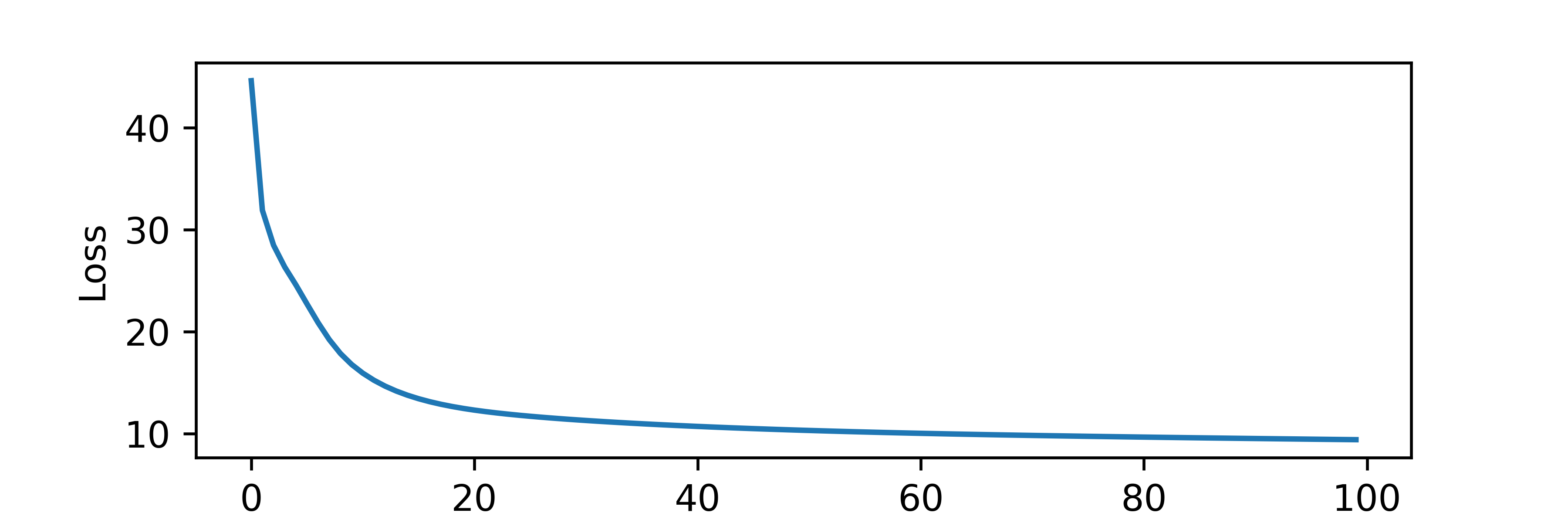
where `l_{rate}` is the learning rate (use 0.3), `err` is the error (difference) between the measured label `y` and the predicted label `p`, and `x_i` is the input feature. Continue for 100 epochs (iteration updates of `\beta`) and plot the loss function.
n_epoch = 100
loss = np.zeros(n_epoch)
beta = [0.0,0.0,0.0]
for epoch in range(n_epoch):
sum_error = 0
for row in train:
x = row[0:-1] # input features
y = row[-1] # output label
p = predict(row, beta)
error = y - p
sum_error += error**2
beta[0] += l_rate * error * p * (1.0 - p)
beta[1] += l_rate * error * p * (1.0 - p) * x[0]
beta[2] += l_rate * error * p * (1.0 - p) * x[1]
loss[epoch] = sum_error
print('Coefficients:',beta)
plt.plot(loss)
plt.xlabel('Epoch')
plt.ylabel('Loss')
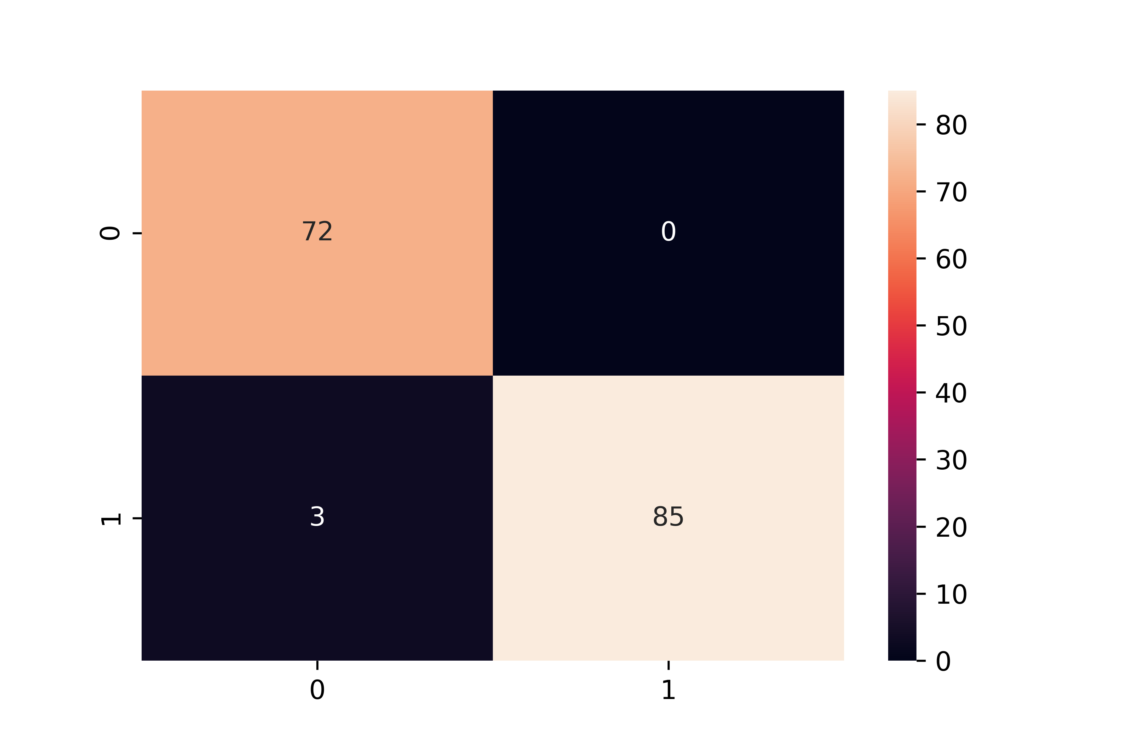
Test the logistic regression model on the remaining 20% the data not used for training.
for row in test:
yhat.append(round(predict(row, beta)))
from sklearn.metrics import confusion_matrix
cmat = confusion_matrix(test[:,-1],yhat)
sns.heatmap(cmat,annot=True)
As a final step, make the code general to accept any number of input features. Test with a random integer for n_features between 3 and 10.
Solutions

Resources
- Logistic Regression on Wikipedia, retrieved 22 Feb 2021.
- Brownlee, J., How To Implement Logistic Regression From Scratch in Python, Machine Learning Mastery, Posted 31 Oct 2016, Updated 11 Dec 2019.
✅ Knowledge Check
1. Which statement best describes the Logistic Regression?
- Incorrect. Logistic Regression, despite its name, is used primarily for classification problems.
- Incorrect. Though it uses a linear combination of features, the prediction is transformed using the sigmoid function.
- Correct. One of the assumptions of Logistic Regression is that all predictors are independent.
- Incorrect. While logistic regression can be adapted for multi-class problems (e.g., using the One-Versus-Rest method), it is inherently binary.
2. In the context of Optical Character Recognition (OCR), what is the primary role of Logistic Regression?
- Incorrect. While OCR does convert images of text to digital format, the role of logistic regression is to classify or recognize characters in those images.
- Correct. Logistic Regression can be used to recognize characters in images of text by being trained on a dataset of images.
- Incorrect. The resolution of scanned documents is not affected by logistic regression. Its role is in classification.
- Incorrect. Noise removal is a preprocessing step and not the primary role of logistic regression in the context of OCR.
Return to Classification Overview