MIMO Model Identification
Multiple Input, Multiple Output (MIMO) systems can be empirically described by several linear dynamic system models. MIMO systems are more complicated than Single Input, Single Output (SISO) systems because of several factors including multivariate interaction, potential co-linearity of inputs, and large data processing requirements. Some common MIMO model forms include:
- Discrete transfer functions (z or q - Time series)
- Continuous transfer functions (s - Laplace variables)
- State space (A,B,C,D - time domain, linear differential equations)
Model identification in these forms typically involves fitting unknown coefficients in the model followed by an analysis to determine how many parameters are statistically significant.
Exercise
The following data set was generated in class from two voltage inputs (u) that changed the temperature (x) of two thermistors from the Arduino Lab.

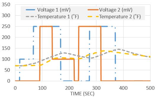
Determine a linear dynamic model that best describes the input to output relationship between voltage and temperature. Compute the steady state gain for each input to output relationship. Data and example script files are posted above in Excel and MATLAB.
Solution (Excel, MATLAB, Python)
Solution (GEKKO Python)
import pandas as pd
import matplotlib.pyplot as plt
# load data and parse into columns
url = 'http://apmonitor.com/do/uploads/Main/tclab_dyn_data2.txt'
data = pd.read_csv(url)
t = data['Time']
u = data[['H1','H2']]
y = data[['T1','T2']]
# generate time-series model
m = GEKKO(remote=False)
# system identification
na = 2 # output coefficients
nb = 2 # input coefficients
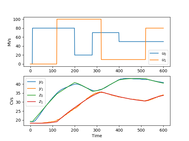
yp,p,K = m.sysid(t,u,y,na,nb,diaglevel=1)
plt.figure()
plt.subplot(2,1,1)
plt.plot(t,u)
plt.legend([r'$u_0$',r'$u_1$'])
plt.ylabel('MVs')
plt.subplot(2,1,2)
plt.plot(t,y)
plt.plot(t,yp)
plt.legend([r'$y_0$',r'$y_1$',r'$z_0$',r'$z_1$'])
plt.ylabel('CVs')
plt.xlabel('Time')
plt.savefig('sysid.png')
plt.show()
import numpy as np
import pandas as pd
import matplotlib.pyplot as plt
# load data and parse into columns
url = 'http://apmonitor.com/do/uploads/Main/tclab_dyn_data2.txt'
data = pd.read_csv(url)
t = data['Time']
u = data[['H1','H2']]
y = data[['T1','T2']]
# generate time-series model
m = GEKKO(remote=False)
# system identification
na = 3 # output coefficients
nb = 4 # input coefficients
yp,p,K = m.sysid(t,u,y,na,nb)
plt.figure()
plt.subplot(2,1,1)
plt.plot(t,u)
plt.legend([r'$H_1$',r'$H_2$'])
plt.ylabel('MVs')
plt.subplot(2,1,2)
plt.plot(t,y)
plt.plot(t,yp)
plt.legend([r'$T_{1meas}$',r'$T_{2meas}$',\
r'$T_{1pred}$',r'$T_{2pred}$'])
plt.ylabel('CVs')
plt.xlabel('Time')
plt.savefig('sysid.png')
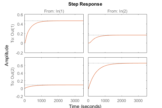
# step test model
yc,uc = m.arx(p)
# steady state initialization
m.options.IMODE = 1
m.solve(disp=False)
# dynamic simulation (step tests)
m.time = np.linspace(0,240,241)
m.options.TIME_SHIFT=0
m.options.IMODE = 4
m.solve(disp=False)
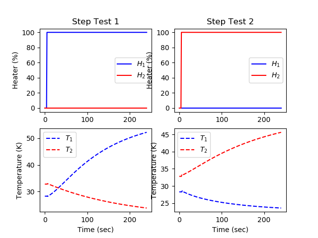
plt.figure()
# step for first MV (Heater 1)
uc[0].value = np.zeros(len(m.time))
uc[0].value[5:] = 100
uc[1].value = np.zeros(len(m.time))
m.solve(disp=False)
plt.subplot(2,2,1)
plt.title('Step Test 1')
plt.plot(m.time,uc[0].value,'b-',label=r'$H_1$')
plt.plot(m.time,uc[1].value,'r-',label=r'$H_2$')
plt.ylabel('Heater (%)')
plt.legend()
plt.subplot(2,2,3)
plt.plot(m.time,yc[0].value,'b--',label=r'$T_1$')
plt.plot(m.time,yc[1].value,'r--',label=r'$T_2$')
plt.ylabel('Temperature (K)')
plt.xlabel('Time (sec)')
plt.legend()
# step for second MV (Heater 2)
uc[0].value = np.zeros(len(m.time))
uc[1].value = np.zeros(len(m.time))
uc[1].value[5:] = 100
m.solve(disp=False)
plt.subplot(2,2,2)
plt.title('Step Test 2')
plt.plot(m.time,uc[0].value,'b-',label=r'$H_1$')
plt.plot(m.time,uc[1].value,'r-',label=r'$H_2$')
plt.ylabel('Heater (%)')
plt.legend()
plt.subplot(2,2,4)
plt.plot(m.time,yc[0].value,'b--',label=r'$T_1$')
plt.plot(m.time,yc[1].value,'r--',label=r'$T_2$')
plt.ylabel('Temperature (K)')
plt.xlabel('Time (sec)')
plt.legend()
plt.show()
References
- Nikbakhsh, S., Hedengren, J.D., Darby, M., Udy, J., Constrained Model Identification Using Open-Equation Nonlinear Optimization, AIChE Spring Meeting, Houston, TX, April 2016. Presentation Abstract