Inverted Pendulum Optimal Control

Design a model predictive controller for an inverted pendulum system with an adjustable cart. Demonstrate that the cart can perform a sequence of moves to maneuver from position y=-1.0 to y=0.0 within 6.2 seconds. Verify that v, $\theta$ , and q are zero before and after the maneuver.

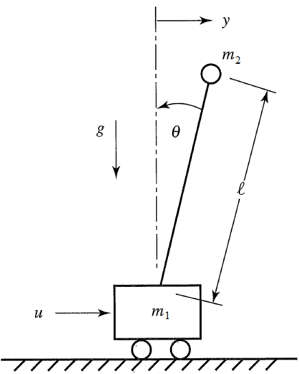
The inverted pendulum is described by the following dynamic equations:

$\begin{bmatrix} \dot y \\ \dot v \\ \dot \theta \\ \dot q \end{bmatrix}=\begin{bmatrix} 0 & 1 & 0 & 0\\ 0 & 0 & -\epsilon & 0\\ 0 & 0 & 0 & 1\\ 0 & 0 & 1 & 0 \end{bmatrix} \begin{bmatrix} y \\ v \\ \theta \\ q \end{bmatrix} + \begin{bmatrix} 0 \\ 1 \\ 0 \\ -1 \end{bmatrix} u$

where u is the force applied to the cart, $\epsilon$ is m₂/(m₁+m₂), y is the position of the cart, v is the velocity of the cart, $\theta$ is the angle of the pendulum relative to the cart, m₁=10, m₂=1, and q is the rate of angle change. Tune the controller to minimize the use of force applied to the cart either in the forward or reverse direction (i.e. minimize fuel consumed to perform the maneuver). Explain the tuning and the optimal solution with appropriate plots that demonstrate that the solution is optimal. The non-inverted pendulum problem and a nonlinear double inverted pendulum are additional examples.

Python (GEKKO) Solution

# Contributed by Everton Colling
import matplotlib.animation as animation
import numpy as np
from gekko import GEKKO

#Defining a model
m = GEKKO()

#################################
#Weight of item
m2 = 1
#################################

#Defining the time, we will go beyond the 6.2s
#to check if the objective was achieved
m.time = np.linspace(0,8,100)
end_loc = int(100.0*6.2/8.0)

#Parameters
m1a = m.Param(value=10)
m2a = m.Param(value=m2)
final = np.zeros(len(m.time))
for i in range(len(m.time)):
if m.time[i] < 6.2:
final[i] = 0
else:
final[i] = 1
final = m.Param(value=final)

#MV
ua = m.Var(value=0)

#State Variables
theta_a = m.Var(value=0)
qa = m.Var(value=0)
ya = m.Var(value=-1)
va = m.Var(value=0)

#Intermediates
epsilon = m.Intermediate(m2a/(m1a+m2a))

#Defining the State Space Model
m.Equation(ya.dt() == va)
m.Equation(va.dt() == -epsilon*theta_a + ua)
m.Equation(theta_a.dt() == qa)
m.Equation(qa.dt() == theta_a -ua)

#Definine the Objectives
#Make all the state variables be zero at time >= 6.2
m.Obj(final*ya**2)
m.Obj(final*va**2)
m.Obj(final*theta_a**2)
m.Obj(final*qa**2)

m.fix(ya,pos=end_loc,val=0.0)
m.fix(va,pos=end_loc,val=0.0)
m.fix(theta_a,pos=end_loc,val=0.0)
m.fix(qa,pos=end_loc,val=0.0)
#Try to minimize change of MV over all horizon
m.Obj(0.001*ua**2)

m.options.IMODE = 6 #MPC
m.solve() #(disp=False)

#Plotting the results
import matplotlib.pyplot as plt
plt.figure(figsize=(12,10))

plt.subplot(221)
plt.plot(m.time,ua.value,'m',lw=2)
plt.legend([r'$u$'],loc=1)
plt.ylabel('Force')
plt.xlabel('Time')
plt.xlim(m.time[0],m.time[-1])

plt.subplot(222)
plt.plot(m.time,va.value,'g',lw=2)
plt.legend([r'$v$'],loc=1)
plt.ylabel('Velocity')
plt.xlabel('Time')
plt.xlim(m.time[0],m.time[-1])

plt.subplot(223)
plt.plot(m.time,ya.value,'r',lw=2)
plt.legend([r'$y$'],loc=1)
plt.ylabel('Position')
plt.xlabel('Time')
plt.xlim(m.time[0],m.time[-1])

plt.subplot(224)
plt.plot(m.time,theta_a.value,'y',lw=2)
plt.plot(m.time,qa.value,'c',lw=2)
plt.legend([r'$\theta$',r'$q$'],loc=1)
plt.ylabel('Angle')
plt.xlabel('Time')
plt.xlim(m.time[0],m.time[-1])

plt.rcParams['animation.html'] = 'html5'

x1 = ya.value
y1 = np.zeros(len(m.time))

#suppose that l = 1
x2 = 1*np.sin(theta_a.value)+x1
x2b = 1.05*np.sin(theta_a.value)+x1
y2 = 1*np.cos(theta_a.value)-y1
y2b = 1.05*np.cos(theta_a.value)-y1

fig = plt.figure(figsize=(8,6.4))
ax = fig.add_subplot(111,autoscale_on=False,\
xlim=(-1.5,0.5),ylim=(-0.4,1.2))
ax.set_xlabel('position')
ax.get_yaxis().set_visible(False)

crane_rail, = ax.plot([-1.5,0.5],[-0.2,-0.2],'k-',lw=4)
start, = ax.plot([-1,-1],[-1.5,1.5],'k:',lw=2)
objective, = ax.plot([0,0],[-0.5,1.5],'k:',lw=2)
mass1, = ax.plot([],[],linestyle='None',marker='s',\
markersize=40,markeredgecolor='k',\
color='orange',markeredgewidth=2)
mass2, = ax.plot([],[],linestyle='None',marker='o',\
markersize=20,markeredgecolor='k',\
color='orange',markeredgewidth=2)
line, = ax.plot([],[],'o-',color='orange',lw=4,\
markersize=6,markeredgecolor='k',\
markerfacecolor='k')
time_template = 'time = %.1fs'
time_text = ax.text(0.05,0.9,'',transform=ax.transAxes)
start_text = ax.text(-1.06,-0.3,'start',ha='right')
end_text = ax.text(0.06,-0.3,'objective',ha='left')

def init():
mass1.set_data([],[])
mass2.set_data([],[])
line.set_data([],[])
time_text.set_text('')
return line, mass1, mass2, time_text

def animate(i):
mass1.set_data([x1[i]],[y1[i]-0.1])
mass2.set_data([x2b[i]],[y2b[i]])
line.set_data([x1[i],x2[i]],[y1[i],y2[i]])
time_text.set_text(time_template % m.time[i])
return line, mass1, mass2, time_text

ani_a = animation.FuncAnimation(fig, animate, \
np.arange(1,len(m.time)), \
interval=40,blit=False,init_func=init)

# requires ffmpeg to save mp4 file
# available from https://ffmpeg.zeranoe.com/builds/
# add ffmpeg.exe to path such as C:\ffmpeg\bin\ in
# environment variables

#ani_a.save('Pendulum_Control.mp4',fps=30)

plt.show()

[$[Get Code]]

Thanks to Everton Colling for the animation code in Python.

APM MATLAB and APM Python Solution

Inverted Pendulum: Solution Files (APM Python and APM MATLAB)

Response with Different Weights

import matplotlib.animation as animation
import numpy as np
from gekko import GEKKO

#Defining a model
m = GEKKO()

#Defining the time, we will go beyond the 6.2s
#to check if the objective was achieved
n = 300
tf = 24.0
m.time = np.linspace(0,tf,n)
end_loc1 = int(n*6.0/tf)
end_loc2 = int(n*12.0/tf)
end_loc3 = int(n*18.0/tf)
end_loc4 = n-1 # end

#################################
#Weight of item
m2 = np.ones(n)
m2[0:end_loc1] = 0.1
m2[end_loc1:end_loc2] = 1.0
m2[end_loc2:end_loc3] = 10.0
m2[end_loc3:end_loc4] = 20.0
#################################

#Parameters
m1a = m.Param(value=10)
m2a = m.Param(value=m2)

#MV
ua = m.Var(value=0)

#State Variables
theta_a = m.Var(value=0)
qa = m.Var(value=0)
ya = m.Var(value=-1)
va = m.Var(value=0)

#Intermediates
epsilon = m.Intermediate(m2a/(m1a+m2a))

#Defining the State Space Model
m.Equation(ya.dt() == va)
m.Equation(va.dt() == -epsilon*theta_a + ua)
m.Equation(theta_a.dt() == qa)
m.Equation(qa.dt() == theta_a -ua)

#Definine the Objectives
#Make all the state variables be zero at endpoints
i = end_loc1
m.fix(ya,pos=i,val=0.0)
m.fix(va,pos=i,val=0.0)
m.fix(theta_a,pos=i,val=0.0)
m.fix(qa,pos=i,val=0.0)

i = end_loc2
m.fix(ya,pos=i,val=-1.0)
m.fix(va,pos=i,val=0.0)
m.fix(theta_a,pos=i,val=0.0)
m.fix(qa,pos=i,val=0.0)

i = end_loc3
m.fix(ya,pos=i,val=0.0)
m.fix(va,pos=i,val=0.0)
m.fix(theta_a,pos=i,val=0.0)
m.fix(qa,pos=i,val=0.0)

i = end_loc4
m.fix(ya,pos=i,val=-1.0)
m.fix(va,pos=i,val=0.0)
m.fix(theta_a,pos=i,val=0.0)
m.fix(qa,pos=i,val=0.0)

#Try to minimize change of MV over all horizon
m.Obj(0.001*ua**2)

m.options.SOLVER = 3
m.options.IMODE = 6 #MPC
m.solve() #(disp=False)

#Plotting the results
import matplotlib.pyplot as plt
plt.figure(figsize=(12,10))

plt.subplot(221)
plt.plot(m.time,ua.value,'m',lw=2)
plt.legend([r'$u$'],loc=1)
plt.ylabel('Force')
plt.xlabel('Time')
plt.xlim(m.time[0],m.time[-1])

plt.subplot(222)
plt.plot(m.time,va.value,'g',lw=2)
plt.legend([r'$v$'],loc=1)
plt.ylabel('Velocity')
plt.xlabel('Time')
plt.xlim(m.time[0],m.time[-1])

plt.subplot(223)
plt.plot(m.time,ya.value,'r',lw=2)
plt.legend([r'$y$'],loc=1)
plt.ylabel('Position')
plt.xlabel('Time')
plt.xlim(m.time[0],m.time[-1])

plt.subplot(224)
plt.plot(m.time,theta_a.value,'y',lw=2)
plt.plot(m.time,qa.value,'c',lw=2)
plt.legend([r'$\theta$',r'$q$'],loc=1)
plt.ylabel('Angle')
plt.xlabel('Time')
plt.xlim(m.time[0],m.time[-1])

plt.rcParams['animation.html'] = 'html5'

x1 = ya.value
y1 = np.zeros(len(m.time))

#suppose that l = 1
x2 = 1*np.sin(theta_a.value)+x1
x2b = 1.05*np.sin(theta_a.value)+x1
y2 = 1*np.cos(theta_a.value)-y1
y2b = 1.05*np.cos(theta_a.value)-y1

fig = plt.figure(figsize=(8,6.4))
ax = fig.add_subplot(111,autoscale_on=False,\
xlim=(-1.8,0.8),ylim=(-0.4,1.2))
ax.set_xlabel('position')
ax.get_yaxis().set_visible(False)

crane_rail, = ax.plot([-2.0,1.0],[-0.2,-0.2],'k-',lw=4)
start, = ax.plot([-1,-1],[-1.5,1.5],'k:',lw=2)
objective, = ax.plot([0,0],[-0.5,1.5],'k:',lw=2)
mass1, = ax.plot([],[],linestyle='None',marker='s',\
markersize=40,markeredgecolor='k',\
color='orange',markeredgewidth=2)
mass2, = ax.plot([],[],linestyle='None',marker='o',\
markersize=20,markeredgecolor='k',\
color='orange',markeredgewidth=2)
line, = ax.plot([],[],'o-',color='orange',lw=4,\
markersize=6,markeredgecolor='k',\
markerfacecolor='k')
time_template = 'time = %.1fs'
time_text = ax.text(0.05,0.9,'',transform=ax.transAxes)
wgt_template = 'weight = %.1f'
wgt_text = ax.text(0.75,0.9,'',transform=ax.transAxes)
start_text = ax.text(-1.06,-0.3,'start',ha='right')
end_text = ax.text(0.06,-0.3,'objective',ha='left')

def init():
mass1.set_data([],[])
mass2.set_data([],[])
line.set_data([],[])
time_text.set_text('')
wgt_text.set_text('')
return line, mass1, mass2, time_text, wgt_text

def animate(i):
mass1.set_data([x1[i]],[y1[i]-0.1])
mass2.set_data([x2b[i]],[y2b[i]])
line.set_data([x1[i],x2[i]],[y1[i],y2[i]])
time_text.set_text(time_template % m.time[i])
wgt_text.set_text(wgt_template % m2[i])
return line, mass1, mass2, time_text, wgt_text

ani_a = animation.FuncAnimation(fig, animate, \
np.arange(1,len(m.time)), \
interval=40,blit=False,init_func=init)

# requires ffmpeg to save mp4 file
# available from https://ffmpeg.zeranoe.com/builds/
# add ffmpeg.exe to path such as C:\ffmpeg\bin\ in
# environment variables
ani_a.save('Pendulum_Control.mp4',fps=30)

plt.show()

[$[Get Code]]

OpenAI Cart Pole

OpenAI has a similar benchmark problem for testing Reinforcement Learning. Similar to the problem above, a pole is attached by a frictionless joint and cart that moves along a track. The cart is controlled by applying a force to the left (action=0) or right (action=1). The pendulum starts upright and a reward of +1 is provided for every timestep that the pole remains upright. The gym returns done=True when the pole is more than 15° from vertical or the cart is more than 2.4 units from the starting location.

import gym
env = gym.make('CartPole-v0')
env.reset()
for i in range(100):
env.render()
# Input:
# Force to the cart with actions: 0=left, 1=right
# Returns:
# obs = cart position, cart velocity, pole angle, rot rate
# reward = +1 for every timestep
# done = True when abs(angle)>15 or abs(cart pos)>2.4
obs,reward,done,info = env.step(env.action_space.sample())
env.close()

[$[Get Code]]

See additional information on Hand Tracking to control the cart position. Reinforcement Learning or Model Predictive Control can also be used to control the cart position (see Additional Reading).

Additional Reading

Bryson, A.E., Dynamic Optimization, Addison-Wesley, 1999.
Balawejder, M., Solving Open AI’s CartPole using Reinforcement Learning, March 31, 2021. Article.
Barto, A.G., Neuronlike adaptive elements that can solve difficult learning control problems, IEEE Transactions on Systems, Man, and Cybernetics, Volume: SMC-13, Issue: 5, 1983. Article
OpenAI, Cart Pole v0 Gym | Documentation | PyTorch RL Solution | TensorFlow RL Solution | Keras RL Solution

Dynamic Optimization