Practice Midterm Exam 2

Problem 1 Solution (Orthogonal Collocation)

# Solution for Orthogonal Collocation on Finite Elements
import numpy as np
from gekko import GEKKO
tf = 10
u = 0.5
x10 = -0.5
x20 = 0.0
m = GEKKO()
x11,x12,x13 = m.Array(m.Var,3)
x21,x22,x23 = m.Array(m.Var,3)
dx11,dx12,dx13 = m.Array(m.Var,3)
dx21,dx22,dx23 = m.Array(m.Var,3)
m.Equations([tf * (0.436*dx11 -0.281*dx12 +0.121*dx13) == x11 - x10, \
tf * (0.614*dx11 +0.064*dx12 +0.046*dx13) == x12 - x10, \
tf * (0.603*dx11 +0.230*dx12 +0.167*dx13) == x13 - x10, \
tf * (0.436*dx21 -0.281*dx22 +0.121*dx23) == x21 - x20, \
tf * (0.614*dx21 +0.064*dx22 +0.046*dx23) == x22 - x20, \
tf * (0.603*dx21 +0.230*dx22 +0.167*dx23) == x23 - x20, \
dx11 == u, \
dx12 == u, \
dx13 == u, \
dx21 == x11**2-u, \
dx22 == x12**2-u, \
dx23 == x13**2-u])
m.solve()
print('States with Orthogonal Collocation')
print('x1 = ', x10, x11.value[0], x12.value[0], x13.value[0])
print('x2 = ', x20, x21.value[0], x22.value[0], x23.value[0])
print(' ')
print('Derivatives with Orthogonal Collocation')
print('dx1/dt = ', dx11.value[0], dx12.value[0], dx13.value[0])
print('dx2/dt = ', dx21.value[0], dx22.value[0], dx23.value[0])
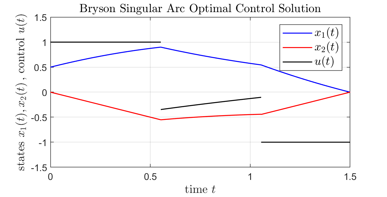
Problem 2 Solution (Bryson Benchmark)
from gekko import GEKKO
import numpy as np
import matplotlib.pyplot as plt
#Build Model ############################
m = GEKKO()
#define time space
nt = 101
m.time = np.linspace(0,1.5,nt)
#Parameters
u = m.MV(value =0, lb = -1, ub = 1)
u.STATUS = 1
u.DCOST = 0.0001 # slight penalty to discourage MV movement
#Variables
x1 = m.Var(value=0.5)
x2 = m.Var(value = 0)
myObj = m.Var()
#Equations
m.Equation(myObj.dt() == 0.5*x1**2)
m.Equation(x1.dt() == u + x2)
m.Equation(x2.dt() == -u)
f = np.zeros(nt)
f[-1] = 1
final = m.Param(value=f)
# Four options for final constraints x1(tf)=0 and x2(tf)=0
option = 2 # best option = 3 (fix endpoints directly)
if option == 1:
# most likely to cause DOF issues because of many 0==0 equations
m.Equation(final*x1 == 0)
m.Equation(final*x2 == 0)
elif option == 2:
# inequality constraint approach is better but there are still
# many inactive equations not at the endpoint
m.Equation((final*x1)**2 <= 0)
m.Equation((final*x2)**2 <= 0)
elif option == 3: #requires GEKKO version >= 0.0.3a2
# fix the value just at the endpoint (best option)
m.fix(x1,pos=nt-1,val=0)
m.fix(x2,pos=nt-1,val=0)
else:
#penalty method ("soft constraint") that may influence the
# optimal solution because there is just one combined objective
# and it may interfere with minimizing myObj
m.Obj(1000*(final*x1)**2)
m.Obj(1000*(final*x2)**2)
m.Obj(myObj*final)
########################################
#Set Global Options and Solve
m.options.IMODE = 6
m.options.NODES = 3
m.options.MV_TYPE = 1
m.options.SOLVER = 1 # APOPT solver
#Solve
m.solve() # (remote=False) for local solution
# Print objective value
print('Objective (myObj): ' + str(myObj[-1]))
########################################
#Plot Results
plt.figure()
plt.plot(m.time, x1.value, 'y:', label = '$x_1$')
plt.plot(m.time, x2.value, 'r--', label = '$x_2$')
plt.plot(m.time, u.value, 'b-', label = 'u')
plt.plot(m.time, myObj.value,'k-',label='Objective')
plt.legend()
plt.show()
% script_BrysonProblem_AnalyticSolution
% thanks to Martin Neuenhofen for providing script
t0 = 0;
tE = 1.5;
t1 = 0.5/tanh(1.5);
% t2 is unique solution of
% (0.5+t1-0.5*t1^2)*exp(t1-t2)==te-t2+0.5*(tE-t2)^2
% in interval [t0,tE].
t2 = 1.05462;
figure;
hold on;
box on;
axis manual;
axis([t0,tE,-1.5,1.5]);
grid on;
% interval [t0,t1]
u = @(t) 1+0*t;
x2 = @(t) -t;
x1 = @(t) 0.5+t-0.5*t.^2;
t = linspace(t0,t1,1000);
plot(t,x1(t),'blue','linewidth',1);
plot(t,x2(t),'red','linewidth',1);
plot(t,u(t) ,'black','linewidth',1);
% interval [t1,t2]
x1_0 = x1(t1);
x2_0 = x2(t1);
x1 = @(t) x1_0 ./ exp(t-t1);
x2 = @(t) x1_0 * sinh(t-t1) + x2_0 * exp(t-t1);
u = @(t) -x1(t)-x2(t);
t = linspace(t1,t2,1000);
plot(t,x1(t),'blue','linewidth',1);
plot(t,x2(t),'red','linewidth',1);
plot(t,u(t) ,'black','linewidth',1);
% interval [t2,tE]
u = @(t) -1+0*t;
x2 = @(t) -1.5+t;
x1 = @(t) (tE-t)+0.5*(tE-t).^2;
t = linspace(t2,tE,1000);
plot(t,x1(t),'blue','linewidth',1);
plot(t,x2(t),'red','linewidth',1);
plot(t,u(t) ,'black','linewidth',1);
legend({'$x_1(t)$','$x_2(t)$','$u(t)$'},...
'Interpreter','LateX','fontsize',12);
title('Bryson Singular Arc Optimal Control Solution',...
'Interpreter','LateX','fontsize',12);
xlabel('time $t$','Interpreter','LateX','fontsize',12);
ylabel('states $x_1(t),x_2(t)$\,, control $u(t)$',...
'Interpreter','LateX','fontsize',12);
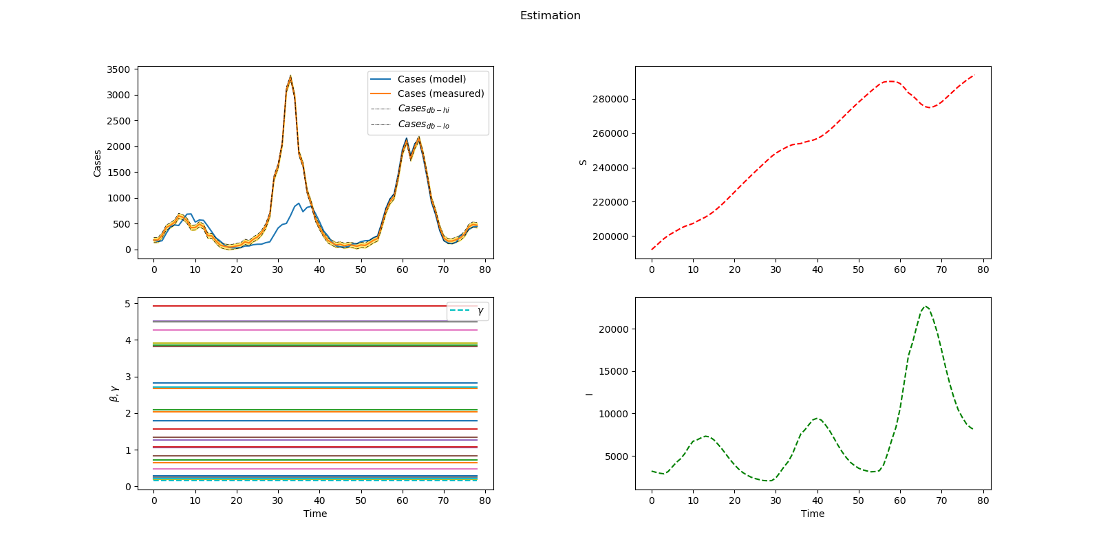
Problem 3 Solution (Infectious Disease)
Thanks to Miriam Medina for providing the GEKKO Python code.
Estimate 26 beta values and gamma
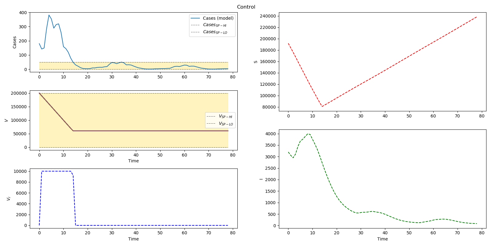
Optimal distribution of measles vaccines
from gekko import GEKKO
import numpy as np
import matplotlib.pyplot as plt
m1 = GEKKO(remote=False)
m2 = GEKKO(remote=False)
m = m1
# known parameters
# number of biweeks in a year
nb = 26
ny = 3 # number of years
biweeks = np.zeros((nb,ny*nb+1))
biweeks[0][0] = 1
for i in range(nb):
for j in range(ny):
biweeks[i][j*nb+i+1] = 1
# write csv data file
tm = np.linspace(0,78,79)
# case data
cases = np.array([180,180,271,423,465,523,649,624,556,420,\
423,488,441,268,260,163,83,60,41,48,65,82,\
145,122,194,237,318,450,671,1387,1617,2058,\
3099,3340,2965,1873,1641,1122,884,591,427,282,\
174,127,84,97,68,88,79,58,85,75,121,174,209,458,\
742,929,1027,1411,1885,2110,1764,2001,2154,1843,\
1427,970,726,416,218,160,160,188,224,298,436,482,468])
data = np.vstack((tm,cases))
data = data.T
np.savetxt('measles_biweek_2.csv',data,delimiter=',',header='time,cases')
#load data from csv
m.time, cases_meas = np.loadtxt('measles_biweek_2.csv', \
delimiter=',',skiprows=1,unpack=True)
m.Vr = m.Param(value = 0)
# Variables
m.N = m.FV(value = 3.2e6)
m.mu = m.FV(value = 7.8e-4)
m.rep_frac = m.FV(value = 0.45)
# beta values (unknown parameters in the model)
m.beta = [m.FV(value=1, lb=0.1, ub=5) for i in range(nb)]
# predicted values
m.S = m.SV(value = 0.06*m.N.value, lb=0,ub=m.N)
m.I = m.SV(value = 0.001*m.N.value, lb=0,ub=m.N)
m.V = m.Var(value = 2e5)
# measured values
m.cases = m.CV(value = cases_meas, lb=0)
# turn on feedback status for CASES
m.cases.FSTATUS = 1
# weight on prior model predictions
m.cases.WMODEL = 0
# meas_gap = deadband that represents level of
# accuracy / measurement noise
db = 100
m.cases.MEAS_GAP = db
for i in range(nb):
m.beta[i].STATUS=1
m.gamma = m.FV(value=0.07)
m.gamma.STATUS = 1
m.gamma.LOWER = 0.05
m.gamma.UPPER = 0.5
m.biweek=[None]*nb
for i in range(nb):
m.biweek[i] = m.Param(value=biweeks[i])
# Intermediate
m.Rs = m.Intermediate(m.S*m.I/m.N)
# Equations
sum_biweek = sum([m.biweek[i]*m.beta[i]*m.Rs for i in range(nb)])
m.Equation(m.S.dt()== -sum_biweek + m.mu*m.N - m.Vr)
m.Equation(m.I.dt()== sum_biweek - m.gamma*m.I)
m.Equation(m.cases == m.rep_frac*sum_biweek)
m.Equation(m.V.dt()==-m.Vr)
# options
m.options.SOLVER = 1
m.options.NODES=3
# imode = 5, dynamic estimation
m.options.IMODE = 5
# ev_type = 1 (L1-norm) or 2 (squared error)
m.options.EV_TYPE = 1
# solve model and print solver output
m.solve()
[print('beta['+str(i+1)+'] = '+str(m.beta[i][0])) \
for i in range(nb)]
print('gamma = '+str(m.gamma.value[0]))
# export data
# stack time and avg as column vectors
my_data = np.vstack((m.time,np.asarray(m.beta),m.gamma))
# transpose data
my_data = my_data.T
# save text file with comma delimiter
beta_str = ''
for i in range(nb):
beta_str = beta_str + ',beta[' + str(i+1) + ']'
header_name = 'time,gamma' + beta_str
##np.savetxt('solution_data.csv',my_data,delimiter=',',\
## header = header_name, comments='')
np.savetxt('solution_data_EVTYPE_'+str(m.options.EV_TYPE)+\
'_gamma'+str(m.gamma.STATUS)+'.csv',\
my_data,delimiter=',',header = header_name)
plt.figure(num=1, figsize=(16,8))
plt.suptitle('Estimation')
plt.subplot(2,2,1)
plt.plot(m.time,m.cases, label='Cases (model)')
plt.plot(m.time,cases_meas, label='Cases (measured)')
if m.options.EV_TYPE==1:
plt.plot(m.time,cases_meas+db/2, 'k-.',\
lw=0.5, label=r'$Cases_{db-hi}$')
plt.plot(m.time,cases_meas-db/2, 'k-.',\
lw=0.5, label=r'$Cases_{db-lo}$')
plt.fill_between(m.time,cases_meas-db/2,\
cases_meas+db/2,color='gold',alpha=.5)
plt.legend(loc='best')
plt.ylabel('Cases')
plt.subplot(2,2,2)
plt.plot(m.time,m.S,'r--')
plt.ylabel('S')
plt.subplot(2,2,3)
[plt.plot(m.time,m.beta[i], label='_nolegend_')\
for i in range(nb)]
plt.plot(m.time,m.gamma,'c--', label=r'$\gamma$')
plt.legend(loc='best')
plt.ylabel(r'$\beta, \gamma$')
plt.xlabel('Time')
plt.subplot(2,2,4)
plt.plot(m.time,m.I,'g--')
plt.xlabel('Time')
plt.ylabel('I')
plt.subplots_adjust(hspace=0.2,wspace=0.4)
name = 'cases_EVTYPE_'+ str(m.options.EV_TYPE) +\
'_gamma' + str(m.gamma.STATUS) + '.png'
plt.savefig(name)
##-----------------------------------------------##
## Control
##-----------------------------------------------##
m = m2
m.time = m1.time
# Variables
N = m.FV(value = 3.2e6)
mu = m.FV(value = 7.8e-4)
rep_frac = m.FV(value = 0.45)
# beta values (unknown parameters in the model)
beta = [m.FV(value = m1.beta[i].NEWVAL) for i in range(nb)]
gamma = m.FV(value = m1.gamma.NEWVAL)
cases = m.CV(value = cases_meas[0],lb=0)
# predicted values
S = m.SV(value=0.06*N, lb=0,ub=N)
I = m.SV(value = 0.001*N, lb=0,ub=N)
V = m.CV(value = 2e5)
Vr = m.MV(value = 0)
cases.STATUS = 1
cases.FSTATUS = 0
cases.TR_INIT = 0
cases.SPHI = 50
cases.SPLO = 0
cases_SPHI = np.full(len(m.time),cases.SPHI)
cases_SPLO = np.full(len(m.time),cases.SPLO)
Vr.STATUS = 1
Vr.UPPER = 1e4
Vr.LOWER = 0
Vr.COST = 1e-5
V.SPHI = 2e5
V.SPLO = 0
V.STATUS = 0
V.TR_INIT = 0
V_SPHI = np.full(len(m.time),V.SPHI)
V_SPLO = np.full(len(m.time),V.SPLO)
biweek=[None]*nb
for i in range(nb):
biweek[i] = m.Param(value=biweeks[i])
# Intermediates
Rs = m.Intermediate(S*I/N)
#Equations
sum_biweek = sum([biweek[i]*beta[i]*Rs for i in range(nb)])
m.Equation(S.dt()== -sum_biweek + mu*N - Vr)
m.Equation(I.dt()== sum_biweek - gamma*I)
m.Equation(cases == rep_frac*sum_biweek)
m.Equation(V.dt() == -Vr)
# options
m.options.SOLVER = 1
# imode = 6, dynamic control
m.options.IMODE = 6
# ctrl_units = 5, time units are in years
m.options.CTRL_UNITS = 5
m.options.CV_TYPE = 1
# solve model and print solver output
m.solve()
[print('beta['+str(i+1)+'] = '+str(beta[i][0]))\
for i in range(nb)]
print('gamma = '+str(gamma.value[0]))
# export data
# stack time and avg as column vectors
my_data = np.vstack((m.time,np.asarray(beta),V,Vr,gamma))
# transpose data
my_data = my_data.T
# save text file with comma delimiter
beta_str = ''
for i in range(nb):
beta_str = beta_str + ',beta[' + str(i+1) + ']'
header_name = 'time,gamma' + beta_str
##np.savetxt('solution_data.csv',my_data,delimiter=',',\
## header = header_name, comments='')
np.savetxt('solution_control_EVTYPE_'+str(m.options.EV_TYPE)+\
'_gamma'+str(gamma.STATUS)+'.csv',\
my_data,delimiter=',',header = header_name)
plt.figure(num=2, figsize=(16,8))
plt.suptitle('Control')
plt.subplot2grid((6,2),(0,0), rowspan=2)
plt.plot(m.time,cases, label='Cases (model)')
plt.plot(m.time,cases_SPHI, 'k-.', lw=0.5,\
label=r'$Cases _{SP-HI}$')
plt.plot(m.time,cases_SPLO, 'k-.', lw=0.5,\
label=r'$Cases _{SP-LO}$')
plt.fill_between(m.time,cases_SPLO,cases_SPHI,\
color='gold',alpha=.25)
plt.legend(loc='best')
plt.ylabel('Cases')
plt.subplot2grid((6,2),(0,1), rowspan=3)
plt.plot(m.time,S,'r--')
plt.ylabel('S')
plt.subplot2grid((6,2),(2,0), rowspan=2)
[plt.plot(m.time,V, label='_nolegend_') for i in range(nb)]
plt.plot(m.time,V_SPHI, 'k-.', lw=0.5,\
label=r'$V _{SP-HI}$')
plt.plot(m.time,V_SPLO, 'k-.', lw=0.5,\
label=r'$V _{SP-LO}$')
plt.fill_between(m.time,V_SPLO,V_SPHI,color='gold',alpha=.25)
plt.legend(loc='best')
plt.ylabel(r'$V$')
plt.xlabel('Time')
plt.subplot2grid((6,2),(3,1),rowspan=3)
plt.plot(m.time,I,'g--')
plt.xlabel('Time')
plt.ylabel('I')
plt.subplot2grid((6,2),(4,0),rowspan=2)
plt.plot(m.time,Vr, 'b--')
plt.ylabel(r'$V_{r}$')
plt.xlabel('Time')
plt.tight_layout()
plt.subplots_adjust(top=0.95,wspace=0.2)
name = 'cases_EVTYPE_'+ str(m.options.EV_TYPE) + '_gamma'+\
str(gamma.STATUS) + '.png'
plt.savefig(name)
plt.show()
See also: Simulation of Infectious Disease Spread
See also Mid-term Practice Exam (2015)