Dynamic Optimization

Moving horizon estimation (MHE) is a type of optimization-based model predictive control algorithm that is used to estimate the states of a system based on noisy measurements. It is an online algorithm that operates in a rolling horizon fashion, meaning that it continually updates the estimates of the states as new measurements become available.

The basic idea of MHE is to minimize the discrepancy between the measured outputs of the system and the outputs predicted by a model of the system, subject to a set of constraints on the states of the system. This optimization problem is often written as follows:

$$\min_{x_k, ..., x_{k+N}} \sum_{i=k}^{k+N} ||y_i - h(x_i)||^2 + \sum_{i=k}^{k+N-1} ||x_{i+1} - f(x_i)||^2$$

subject to:

$$x_k = x_{k,0}$$

$$g_j(x_i) \leq 0 \quad (j=1,2,...,m)$$

where `x_k,\ldots, x_{k+N}` are the states of the system at each time step in the horizon, y_i is the measured output at time i, h(x_i) is the model prediction of the output at time i, f(x_i) is the model prediction of the state at time i+1 given the state at time i, x_k,0 is the initial estimate of the state at time k, and g_j(x_i) are the constraints on the states at time i. Additional optimization forms are discussed in Estimator Objectives.

The optimization problem is solved using an optimization algorithm, such as the interior point method, at each time step as new measurements become available. The solution of the optimization problem gives the estimates of the states of the system for the current time step and the next few time steps in the horizon. The horizon is then shifted forward by one time step and the process is repeated.

MHE can be useful for systems that are subject to noise or disturbance, as it allows the model to adapt to these changes and maintain accurate estimates of the states. It is also useful for systems with constraints on the states, as the constraints can be incorporated into the optimization problem.

Dynamic models constructed with equations that describe physical phenomena may need to be tuned by adjusting parameters so that predicted outputs match with experimental data. Physical models are based on the underlying physical principles that govern the problem and result from expressions such as a force or momentum balance and may include quantities such as velocity, acceleration, and position. Other quantities of interest may include anything that changes with respect to time such as reactor composition, temperature, mole fraction, etc. Mathematical models likely contain both physical and experimental elements. This section shows how to reconcile experimental data with the physical model through parameter estimation.

Moving Horizon Estimation (MHE) uses dynamic optimization and a backward time horizon of measurements to optimally adjust parameters and states. The data may include noise (random fluctuations), drift (gradual departure from true values), outliers (sudden and temporary departure from true values), or other inaccuracies. Nonlinear programming solvers are employed to numerically converge the dynamic optimization problem.

Exercise

Objective: Design an estimator to predict an unknown parameter and state variable. Use a model of the reactor and implement the estimator to detect the current states (temperature and concentration) as well as the unmeasured heat transfer coefficient (U). Estimated time: 2-3 hours.

CSTR Source Files

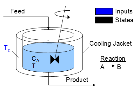
A reactor is used to convert a hazardous chemical A to an acceptable chemical B in waste stream before entering a nearby lake. This particular reactor is dynamically modeled as a Continuously Stirred Tank Reactor (CSTR) with a simplified kinetic mechanism that describes the conversion of reactant A to product B with an irreversible and exothermic reaction. It is desired to maintain the temperature at a constant setpoint that maximizes the destruction of A (highest possible temperature). First, however, an estimator must predict the concentration of A because there is no direct measurement of this quantity. The reaction kinetics and dynamic equations are well-known but there is a parameter in the model, the heat transfer coefficient UA, that is unknown.

Design an estimator to predict the concentration of A leaving the reactor and the heat transfer coefficient UA from the measured reactor temperature T and jacket temperature T_c. See a related CSTR case study for details on the model.

Solution

The estimator can be any type such as a Kalman filter, Extended Kalman filter, Unscented Kalman Filter (particle filter), or an observer that can detect the states (T and Ca) along with the unknown parameter (U). The following solutions demonstrate an implementation of Moving Horizon Estimation.

CSTR MHE Solution in MATLAB

CSTR MHE Solution in Python

CSTR MHE Solution in Simulink

References

1. Haseltine, E.L., Rawlings, J.B., Critical Evaluation of Extended Kalman Filtering and Moving-Horizon Estimation, Industrial & Engineering Chemistry Research 2005 44 (8), 2451-2460, DOI: 10.1021/ie034308l Preprint, Article
2. Spivey, B.J., Hedengren, J.D., Edgar, T.F., Constrained Nonlinear Estimation for Industrial Process Fouling, Industrial & Engineering Chemistry Research 2010 49 (17), 7824-7831, DOI: 10.1021/ie9018116 Article
3. Hedengren, J. D., Eaton, A. N., Overview of Estimation Methods for Industrial Dynamic Systems, Optimization and Engineering, Springer, Vol 18 (1), 2017, pp. 155-178, DOI: 10.1007/s11081-015-9295-9. Preprint, Article