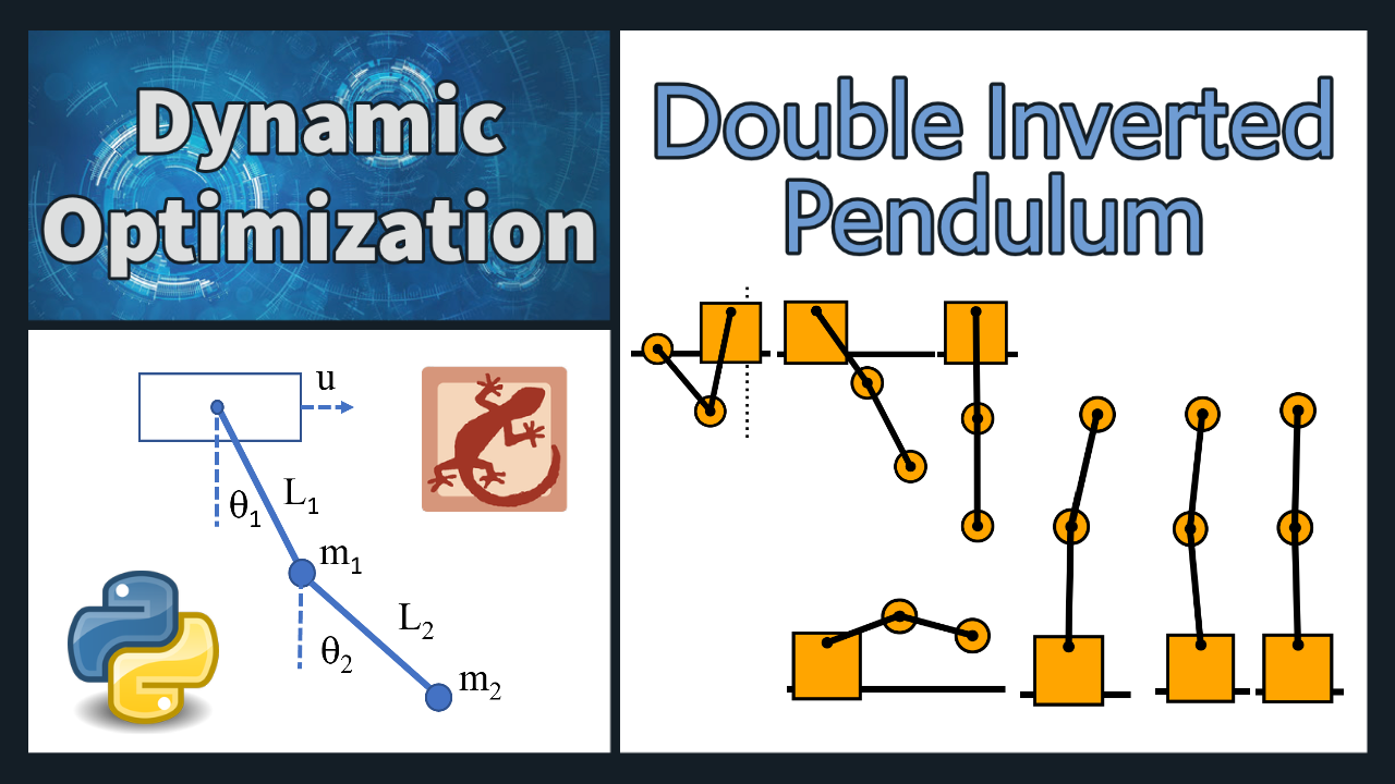
Double Inverted Pendulum Control
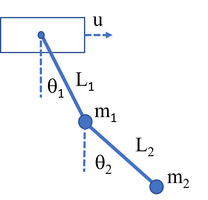
A double inverted pendulum is a dynamic system consisting of two pendulums, where the second pendulum is attached to the first pendulum. The motion of the system is governed by a set of equations derived using Lagrangian mechanics. The Lagrangian is the difference between the kinetic and potential energies of the system and is given by: L = T - V where T is the kinetic energy and V is the potential energy. For the double inverted pendulum, the kinetic energy T is given by the sum of the kinetic energies of each pendulum. The potential energy V is the sum of the gravitational potential energies of each pendulum.
Using the Lagrangian, the equations of motion for the double inverted pendulum are:
$$\begin{aligned}&(m_1 + m_2)L_1\ddot{\theta}_1 +m_2L_2\ddot{\theta}_2\cos(\theta_1-\theta_2) +m_2L_2\dot{\theta}_2^2\sin(\theta_1-\theta_2)\cos(\theta_1-\theta_2) \\ &\quad + g(m_1 + m_2)\sin(\theta_1) = 0 \\ &m_2L_2\ddot{\theta}_2 + m_2L_1\ddot{\theta}_1\cos(\theta_1-\theta_2) - m_2L_1\dot{\theta}_1^2\sin(\theta_1-\theta_2) + gm_2\sin(\theta_2) = 0 \end{aligned}$$
In these equations, `m_1` and `m_2` are the masses of the first and second pendulums, `L_1` and `L_2` are the lengths of the first and second pendulums, `\theta_1` and `\theta_2` are the angles that the first and second pendulums make with the vertical, `\ddot{\theta}_1` and `\ddot{\theta}_2` represent the second derivative of the angles with respect to time, `\dot{\theta}_1` and `\dot{\theta}_2` represent the derivative of the angles with respect to time, `g` is the acceleration due to gravity. These equations describe the motion of the double inverted pendulum and can be used to simulate and control the system. The system is known to be highly nonlinear, and the behavior is chaotic and unpredictable with unmeasured disturbances and friction, making it a popular topic for research in control theory and nonlinear dynamics. For a derivation of the equations of motion, see derivation summary by Mehmet Han İnyayla. For a linearized single inverted pendulum, see the Inverted Pendulum Problem.
Exercise 1: Swing Up
Design a controller for the double inverted pendulum system that can swing the pendulum up from a rest position to the upright vertical position and keep it balanced at the upright position. The controller must be able to control the motion of both pendulums and apply forces to the cart to stabilize it.
One possible approach to designing the controller is to use a model-based control technique such as LQR (Linear Quadratic Regulator) or MPC (Model Predictive Control). These techniques use a mathematical model of the system to design a controller that minimizes a cost function while satisfying constraints on the system. Another approach is to use a reinforcement learning algorithm to learn the optimal control policy directly from interactions with the system. This approach has been shown to be effective for controlling complex and nonlinear systems such as the double inverted pendulum.
Regardless of the approach, the controller should be tested and validated using simulations and experiments to ensure the effectiveness and robustness. The performance of the controller can be evaluated based on metrics such as settling time, overshoot, and tracking error. The design of the controller should take into account the nonlinear dynamics of the system, which makes the system highly unstable and difficult to control. For a physical system, the controller must also be robust to disturbances and uncertainties in the system, such as friction and sensor noise.
#Inverted Double Pendulum Control Optimization
#Adapted from code by Everton Colling
import math
import matplotlib
matplotlib.use("TkAgg")
import matplotlib.animation as animation
import numpy as np
from gekko import GEKKO
#Defining a model
m = GEKKO(remote=True)
#################################
#Define initial and final conditions and limits
pi = math.pi;
x0 = 0; xdot0 = 0
q10 = pi; q1dot0 = 0 #0=vertical, pi=inverted
q20 = pi; q2dot0 = 0 #0=vertical, pi=inverted
xf = 0; xdotf = 0
q1f = 0; q1dotf = 0
q2f = 0; q2dotf = 0
xmin = -2; xmax = 2
umin = -10; umax = 10
#Defining the time parameter (0, 1)
N = 100
t = np.linspace(0,1,N)
m.time = t
#Final time
TF = m.FV(12,lb=2,ub=25); TF.STATUS = 1
end_loc = len(m.time)-1
final = np.zeros(len(m.time))
for i in range(N):
if i >=(N-2):
final[i] = 1000
#final[end_loc] = 100
final = m.Param(value=final)
#Parameters
mc = m.Param(value=1) #cart mass
m1 = m.Param(value=.1) #link 1 mass
m2 = m.Param(value=.1) #link 2 mass
L1 = m.Param(value=.5) #link 1 length
LC1 = m.Param(value=.25) #link 1 CM pos
L2 = m.Param(value=.5) #link 1 length
LC2 = m.Param(value=.25) #link 1 CM pos
I1 = m.Param(value=.01) #link 1 MOI
I2 = m.Param(value=.01) #link 2 MOI
g = m.Const(value=9.81) #gravity
Bc = m.Const(value=.5) #cart friction
B1 = m.Const(value=.001) #link 1 friction
B2 = m.Const(value=.001) #link 2 friction
#MV
u = m.MV(lb=umin,ub=umax); u.STATUS = 1
#State Variables
x, xdot, q1, q1dot, q2, q2dot = m.Array(m.Var, 6)
x.value = x0; xdot.value = xdot0
q1.value = q10; q1dot.value = q1dot0
q2.value = q20; q2dot.value = q2dot0
x.LOWER = xmin; x.UPPER = xmax
#Intermediates
h1 = m.Intermediate(mc + m1 + m2)
h2 = m.Intermediate(m1*LC1 + m2*L1)
h3 = m.Intermediate(m2*LC2)
h4 = m.Intermediate(m1*LC1**2 + m2*L1**2 + I1)
h5 = m.Intermediate(m2*LC2*L1)
h6 = m.Intermediate(m2*LC2**2 + I2)
h7 = m.Intermediate(m1*LC1*g + m2*L1*g)
h8 = m.Intermediate(m2*LC2*g)
M = np.array([[h1, h2*m.cos(q1), h3*m.cos(q2)],
[h2*m.cos(q1), h4, h5*m.cos(q1-q2)],
[h3*m.cos(q2), h5*m.cos(q1-q2), h6]])
C = np.array([[Bc, -h2*q1dot*m.sin(q1), -h3*q2dot*m.sin(q2)],
[0, B1+B2, h5*q2dot*m.sin(q1-q2)-B2],
[0, -h5*q1dot*m.sin(q1-q2)-B2, B2]])
G = np.array([0, -h7*m.sin(q1), -h8*m.sin(q2)])
U = np.array([u, 0, 0])
DQ = np.array([xdot, q1dot, q2dot])
CDQ = C@DQ
b = np.array([xdot.dt()/TF, q1dot.dt()/TF, q2dot.dt()/TF])
Mb = M@b
#Defining the State Space Model
m.Equations([(Mb[i] == U[i] - CDQ[i] - G[i]) for i in range(3)])
m.Equation(x.dt()/TF == xdot)
m.Equation(q1.dt()/TF == q1dot)
m.Equation(q2.dt()/TF == q2dot)
m.Obj(final*(x-xf)**2)
m.Obj(final*(xdot-xdotf)**2)
m.Obj(final*(q1-q1f)**2)
m.Obj(final*(q1dot-q1dotf)**2)
m.Obj(final*(q2-q2f)**2)
m.Obj(final*(q2dot-q2dotf)**2)
#Try to minimize final time
m.Obj(TF)
m.options.IMODE = 6 #MPC
m.options.SOLVER = 3 #IPOPT
m.solve()
m.time = np.multiply(TF, m.time)
print('Final time: ', TF.value[0])
print(q1dot.value)
#Plotting the results
import matplotlib.pyplot as plt
plt.close('all')
fig1 = plt.figure()
fig2 = plt.figure()
ax1 = fig1.add_subplot()
ax2 = fig2.add_subplot(321)
ax3 = fig2.add_subplot(322)
ax4 = fig2.add_subplot(323)
ax5 = fig2.add_subplot(324)
ax6 = fig2.add_subplot(325)
ax7 = fig2.add_subplot(326)
ax1.plot(m.time,u.value,'m',lw=2)
ax1.legend([r'$u$'],loc=1)
ax1.set_title('Control Input')
ax1.set_ylabel('Force (N)')
ax1.set_xlabel('Time (s)')
ax1.set_xlim(m.time[0],m.time[-1])
ax1.grid(True)
ax2.plot(m.time,x.value,'r',lw=2)
ax2.set_ylabel('Position (m)')
ax2.set_xlabel('Time (s)')
ax2.legend([r'$x$'],loc='upper left')
ax2.set_xlim(m.time[0],m.time[-1])
ax2.grid(True)
ax2.set_title('Cart Position')
ax3.plot(m.time,xdot.value,'g',lw=2)
ax3.set_ylabel('Velocity (m/s)')
ax3.set_xlabel('Time (s)')
ax3.legend([r'$xdot$'],loc='upper left')
ax3.set_xlim(m.time[0],m.time[-1])
ax3.grid(True)
ax3.set_title('Cart Velocity')
q1alt = np.zeros((N,1)); q2alt = np.zeros((N,1));
for i in range(N):
q1alt[i] = q1.value[i] + math.pi/2
q2alt[i] = q2.value[i] + math.pi/2
ax4.plot(m.time,q1alt,'r',lw=2)
ax4.set_ylabel('Angle (Rad)')
ax4.set_xlabel('Time (s)')
ax4.legend([r'$q1$'],loc='upper left')
ax4.set_xlim(m.time[0],m.time[-1])
ax4.grid(True)
ax4.set_title('Link 1 Position')
ax5.plot(m.time,q1dot.value,'g',lw=2)
ax5.set_ylabel('Angular Velocity (Rad/s)')
ax5.set_xlabel('Time (s)')
ax5.legend([r'$q1dot$'],loc='upper right')
ax5.set_xlim(m.time[0],m.time[-1])
ax5.grid(True)
ax5.set_title('Link 1 Velocity')
ax6.plot(m.time,q2alt,'r',lw=2)
ax6.set_ylabel('Angle (Rad)')
ax6.set_xlabel('Time (s)')
ax6.legend([r'$q2$'],loc='upper left')
ax6.set_xlim(m.time[0],m.time[-1])
ax6.grid(True)
ax6.set_title('Link 2 Position')
ax7.plot(m.time,q2dot.value,'g',lw=2)
ax7.set_ylabel('Angular Velocity (Rad/s)')
ax7.set_xlabel('Time (s)')
ax7.legend([r'$q2dot$'],loc='upper right')
ax7.set_xlim(m.time[0],m.time[-1])
ax7.grid(True)
ax7.set_title('Link 2 Velocity')
plt.rcParams['animation.html'] = 'html5'
x1 = x.value
y1 = np.zeros(len(m.time))
x2 = L1.value*np.sin(q1.value)+x1
x2b = (1.05*L1.value[0])*np.sin(q1.value)+x1
y2 = L1.value[0]*np.cos(q1.value)+y1
y2b = (1.05*L1.value[0])*np.cos(q1.value)+y1
x3 = L2.value[0]*np.sin(q2.value)+x2
x3b = (1.05*L2.value[0])*np.sin(q2.value)+x2
y3 = L2.value[0]*np.cos(q2.value)+y2
y3b = (1.05*L2.value[0])*np.cos(q2.value)+y2
fig = plt.figure(figsize=(8,6.4))
ax = fig.add_subplot(111,autoscale_on=False,\
xlim=(-2.5,2.5),ylim=(-1.25,1.25))
ax.set_xlabel('position')
ax.get_yaxis().set_visible(False)
crane_rail, = ax.plot([-2.5,2.5],[-0.2,-0.2],'k-',lw=4)
start, = ax.plot([-1.5,-1.5],[-1.5,1.5],'k:',lw=2)
objective, = ax.plot([1.5,1.5],[-1.5,1.5],'k:',lw=2)
mass1, = ax.plot([],[],linestyle='None',marker='s',\
markersize=40,markeredgecolor='k',\
color='orange',markeredgewidth=2)
mass2, = ax.plot([],[],linestyle='None',marker='o',\
markersize=20,markeredgecolor='k',\
color='orange',markeredgewidth=2)
mass3, = ax.plot([],[],linestyle='None',marker='o',\
markersize=20,markeredgecolor='k',\
color='orange',markeredgewidth=2)
line12, = ax.plot([],[],'o-',color='black',lw=4,\
markersize=6,markeredgecolor='k',\
markerfacecolor='k')
line23, = ax.plot([],[],'o-',color='black',lw=4,\
markersize=6,markeredgecolor='k',\
markerfacecolor='k')
time_template = 'time = %.1fs'
time_text = ax.text(0.05,0.9,'',transform=ax.transAxes)
#start_text = ax.text(-1.1,-0.3,'start',ha='right')
#end_text = ax.text(1.0,-0.3,'end',ha='left')
def init():
mass1.set_data([],[])
mass2.set_data([],[])
mass3.set_data([],[])
line12.set_data([],[])
line23.set_data([],[])
time_text.set_text('')
return line12, line23, mass1, mass2, mass3, time_text
def animate(i):
mass1.set_data([x1[i]], [y1[i]-0.1])
mass2.set_data([x2[i]], [y2[i]])
mass3.set_data([x3[i]], [y3[i]])
line12.set_data([x1[i],x2[i]],[y1[i],y2[i]])
line23.set_data([x2[i],x3[i]],[y2[i],y3[i]])
time_text.set_text(time_template % m.time[i])
return line12, line23, mass1, mass2, mass3, time_text
ani_a = animation.FuncAnimation(fig, animate, \
np.arange(len(m.time)), \
interval=40,init_func=init) #blit=False,
ani_a.save('Pendulum_Swing_Up.mp4',fps=30)
plt.show()
#Export Data
import csv
with open('U.csv', 'w', newline = '') as csvfile:
my_writer = csv.writer(csvfile, delimiter = ' ')
for i in range(N):
input = np.array((m.time[i], u.value[i], x.value[i], q1.value[i], q2.value[i]))
my_writer.writerow(input)
csvfile.close
Exercise 2: Horizontal Shift
Design a model predictive controller for an double inverted pendulum system with an adjustable cart. Demonstrate that the cart can perform a sequence of moves to maneuver from position y=-1.5 to y=1.5. Verify that velocities are zero and angles are upright before and after the maneuver.
Change the initial and final conditions section of the code.
q10 = 0; q1dot0 = 0 #0=vertical, pi=inverted
q20 = 0; q2dot0 = 0 #0=vertical, pi=inverted
xf = 1.5; xdotf = 0
Thanks to Theodore Bounds for providing the source code.