Video Data Analysis


Electro-optical sensors detect and convert light into an electronic signal. Digital cameras are a source of visual information that can be translated into quantifiable information for data-driven engineering. Video frames are used to analyze flare stacks for pollutants, navigate self-driving cars, detect intruders, and build 3D photogrammetric models. This tutorial is a demonstration of video data analysis with an application to running form analysis.
Install OpenCV
Install OpenCV once and restart the kernel to use the package. Uncomment this cell to install OpenCV. It can be removed if installation is successful.
Packages are installed once, not every time the program runs. See information on how to Install Python Packages.
Import Video Libraries
Once packages are installed, a next step is to import libraries for video analysis. OpenCV, scikit-image, Pillow, and Numpy are standard libraries in Python for working with image and video data.
import matplotlib.pyplot as plt
import cv2
Download Video File and View Video
The urllib package downloads files from a web address. Another video can be substituted by placing the video in the run directory and changing the filename f='runner.mp4'
f = 'runner.mp4'
url = 'http://apmonitor.com/dde/uploads/Main/'+f
urllib.request.urlretrieve(url,f)
View Video
The example is 22 frames with a 30 frames/sec (fps) video of a runner in a 0.7 sec video segment. View the video in an IPython Notebook or else open the video from the run directory with another video viewing application.
Video(f,width=550)
Import Video File
OpenCV is used to import the video and retrieve information such as the dimensions (pixels) of the video. The video frames are stored as a collection of images with dimensions (h,w,3) with the 3 as a the Blue, Green, and Red (BGR) elements.
v = cv2.VideoCapture(f)
w = int(v.get(cv2.CAP_PROP_FRAME_WIDTH))
h = int(v.get(cv2.CAP_PROP_FRAME_HEIGHT))
v.release()
print('Dimensions:',w,h)
Dimensions: 1920 1080
Read Frames
The individual frames of the video are stored as list img. It is possible to transfer the entire contents of the video to memory in this example, but longer videos hold and process only one frame of the video in memory at a time to stay within memory limits.
v = cv2.VideoCapture(f)
while v.isOpened():
success, image = v.read()
if success:
img.append(image)
else:
break
v.release()
print('Frames Read:',len(img))
Frames Read: 22
Convert BGR (OpenCV) to RGB Format
Some applications (OpenCV) work in BGR format while others (Matplotlib, MediaPipe, Pillow) work in RBG format. Use the cv2.cvtColor() function to convert between BGR and RGB or else use the command img[i] = im[:,:,[2,1,0]] to rearrange the color order.
img[i] = cv2.cvtColor(im, cv2.COLOR_BGR2RGB)
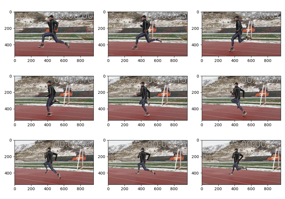
Diplay First 9 Frames
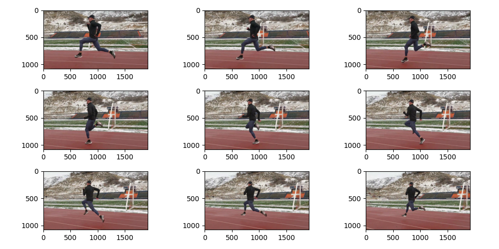
Matplotlib subplots show the first 9 frames of the 22 frame video with plt.imshow(). The plot axes show how the matrices are ordered with x=0 and y=0 as the top left corner of the image.
for i in range(9):
plt.subplot(3,3,i+1); plt.imshow(img[i])
plt.tight_layout()
Get Pose with Deep Learning
Now that the video frames are imported, data can be extracted from the video. In this case, the pose information of the runner is extracted with pretrained MediaPipe or YOLO detection of pose.
import urllib
# Download video file
f = 'runner.mp4'
url = 'http://apmonitor.com/dde/uploads/Main/' + f
urllib.request.urlretrieve(url, f)
# Load YOLO pose estimation model
model = YOLO('yolo11x-pose.pt')
# video saved in runs/pose/track/ as runner.avi
results = model.track(source=f, show=True, save=True)
Install ultralytics if needed.
Once ultralytics is installed, it may be required to restart the kernel. After the kernel is restarted, import the ultralytics YOLO package.
import pandas as pd
from ultralytics import YOLO
import matplotlib.pyplot as plt
import urllib.request
# Download video file
f = 'runner.mp4'
url = 'http://apmonitor.com/dde/uploads/Main/' + f
urllib.request.urlretrieve(url, f)
# Load YOLO pose estimation model
model = YOLO('yolo11x-pose.pt')
# Import the .mp4 video
video = cv2.VideoCapture(f)
# Get video dimensions and FPS
frame_width = int(video.get(cv2.CAP_PROP_FRAME_WIDTH))
frame_height = int(video.get(cv2.CAP_PROP_FRAME_HEIGHT))
fps = int(video.get(cv2.CAP_PROP_FPS))
print('Dimensions:', frame_width, frame_height, 'FPS:', fps)
# Read video frames
frames = []
while video.isOpened():
success, frame = video.read()
if success:
frames.append(frame)
else:
break
video.release()
print('Frames Read:', len(frames))
# Initialize DataFrame for storing results
columns = ['frame', 'Lshldr_x', 'Lshldr_y', 'Lshldr_conf',
'Lhip_x', 'Lhip_y', 'Lhip_conf',
'Lknee_x', 'Lknee_y', 'Lknee_conf']
pose_data = pd.DataFrame(columns=columns)
# Define skeleton connections (COCO format example)
connections = [
(5, 6), (5, 11), (11, 13), (13, 15), # Left Shoulder to Left Hip, Left Knee, Left Ankle
(6, 12), (12, 14), (14, 16), # Right Shoulder to Right Hip, Right Knee, Right Ankle
(5, 7), (7, 9), (6, 8), (8, 10), # Arms (Shoulder to Elbow to Wrist)
(5, 6) # Shoulders
]
# Prepare video writer
output_file = 'processed_runner.mp4'
fourcc = cv2.VideoWriter_fourcc(*'mp4v')
output_video = cv2.VideoWriter(output_file, fourcc, fps, (frame_width, frame_height))
# Process each frame for pose keypoints
for frame_index, frame in enumerate(frames):
results = model(frame)
# Extract keypoints from results
if results:
keypoints = results[0].keypoints.data[0].cpu().numpy() # Convert to numpy array
# Assuming keypoints order matches COCO format:
# Indices for Left Shoulder, Left Hip, Left Knee (COCO indices: 5, 11, 13)
l_shoulder = keypoints[5]
l_hip = keypoints[11]
l_knee = keypoints[13]
# Append data to DataFrame
new_row = pd.DataFrame([{
'frame': frame_index,
'Lshldr_x': l_shoulder[0], 'Lshldr_y': l_shoulder[1], 'Lshldr_conf': l_shoulder[2],
'Lhip_x': l_hip[0], 'Lhip_y': l_hip[1], 'Lhip_conf': l_hip[2],
'Lknee_x': l_knee[0], 'Lknee_y': l_knee[1], 'Lknee_conf': l_knee[2]
}])
pose_data = pd.concat([pose_data, new_row], ignore_index=True)
# Draw skeleton lines
for conn in connections:
start_idx, end_idx = conn
if keypoints[start_idx][2] > 0.5 and keypoints[end_idx][2] > 0.5: # Confidence threshold
start_point = (int(keypoints[start_idx][0]), int(keypoints[start_idx][1]))
end_point = (int(keypoints[end_idx][0]), int(keypoints[end_idx][1]))
cv2.line(frame, start_point, end_point, color=(255, 0, 0), thickness=2)
# Draw keypoints
for kpt in keypoints:
if kpt[2] > 0.5: # Confidence threshold
x, y = int(kpt[0]), int(kpt[1])
cv2.circle(frame, (x, y), radius=3, color=(0, 255, 0), thickness=-1)
# Write the processed frame to the video
output_video.write(frame)
# Release video writer and save pose data
output_video.release()
pose_data.to_csv(f'{f}.csv', index=False)
print(f"Processed video saved as {output_file}")
Install MediaPipe if needed.
Once MediaPipe is installed, it may be required to restart the kernel. After the kernel is restarted, import the MediaPipe packages and rename some of the imports to shorten the name.
import mediapipe as mp
mpds = mp.solutions.drawing_styles
mpdu = mp.solutions.drawing_utils
mpp = mp.solutions.pose
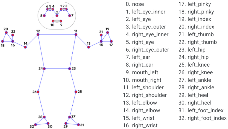
A Pandas DataFrame is created to store the pose information as (X,Y,Z) coordinates and a visibility rating (0-1) for the left shoulder, left hip, and left knee. There are a total of 33 possible landmarks reported with corresponding coordinates and visibility. Only a subset are recorded and exported to a CSV file as an example. All 33 points are plotted on the runner by augmenting the image with the draw_landmarks function. See MediaPipe Pose for additional information.
x = {'frame':[],\
'Lshldr_x':[],'Lshldr_y':[],'Lshldr_z':[],'Lshldr_v':[],\
'Lhip_x':[],'Lhip_y':[],'Lhip_z':[],'Lhip_v':[],\
'Lknee_x':[],'Lknee_y':[],'Lknee_z':[],'Lknee_v':[]}
s = pd.DataFrame(x)
with mpp.Pose(
min_detection_confidence=0.2,
static_image_mode=False,
model_complexity=2,
smooth_landmarks=True,
enable_segmentation=False,
smooth_segmentation=False,
min_tracking_confidence=0.2) as pose:
for i,im in enumerate(img):
im2 = cv2.cvtColor(im, cv2.COLOR_RGB2BGR)
results = pose.process(im2)
if not results.pose_landmarks:
continue
# draw landmarks on frame
mpdu.draw_landmarks(
im2,results.pose_landmarks,
mpp.POSE_CONNECTIONS,
landmark_drawing_spec=mpds.get_default_pose_landmarks_style())
img[i] = im2
# store values in dataframe
row = [i]
for j,lm in enumerate(results.pose_landmarks.landmark):
if j in [11,23,25]:
row.extend([lm.x,lm.y,lm.z,lm.visibility])
s.loc[i] = row
s.to_csv(f+'.csv')
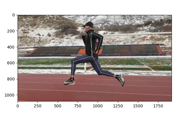
plt.imshow(img[0][:,:,[2,1,0]])
plt.tight_layout()
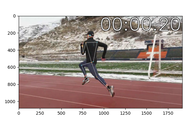
Modify Frames: Add Text
Once the landmarks are drawn on the runner and pose information stored, a next step is to add text to the frames as a timer. The timer letters need to be visible with dark or light backgrounds so the numbers are white with a black outline. This effect is created with a thicker black font followed by a thinner white font on top.
for i,im in enumerate(img):
tm = i/30.0
dm,ds = divmod(tm, 60)
str_time = '{0:02d}:{1:05.2f}'.format(int(dm), ds)
# large text at the top with timer
black = (0,0,0); white = (255,255,255)
cv2.putText(im,str_time,(950,170), \
font, 6.8,black,20,cv2.LINE_AA)
cv2.putText(im,str_time,(950,170), \
font, 6.8,white,10,cv2.LINE_AA)
plt.imshow(img[6][:,:,[2,1,0]])
plt.tight_layout()
Modify Frames: Resize
The frame size is adjusted with the cv2.resize() function with a scaling factor of 0.5. Each dimension of the image is reduced by 50% to reduce overall storage to 25% of the original images.
for i,im in enumerate(img):
img[i] = cv2.resize(im,None,fx=scale,fy=scale)
Get New Frame Size
The prior dimensions are 1920p (width) x 1080p (height) = 2,073,600 pixels and the new dimensions are 960p (width) x 540p (height) = 518,400 pixels. Each frame is stored as a 3D numpy array with height (h), width (w), and color (c) information.
print('New Dimensions:',h,w)
New Dimensions: 540 960
Display Resized Frames
The newly resized images are now displayed in RGB format with img[i][:,:,[2,1,0]] to swap the Blue and Red when converting from OpenCV to Matplotlib formats.
for i in range(9):
plt.subplot(3,3,i+1); plt.imshow(img[i][:,:,[2,1,0]])
plt.tight_layout()
Export Video File
The individual frames are now put back into a video format. Possible formats are MOV, MP4, AVI, WEBM, and others. The WEBM format is used in this case to maximize the potential browser compatibility.
# common formats:
# avi with XVID (fast writing, larger file)
# mp4 with MP4V or H264 (not compatible with some browsers)
# webm with vp80 (slow writing, smaller file)
out = cv2.VideoWriter(fnew,\
cv2.VideoWriter_fourcc(*'vp80'),5,(w,h))
for im in img:
out.write(im)
out.release()
Display Modified Video
The new video with timer and pose information is viewed in slow motion with 5 fps for a total of 4.2 sec. The length of the video increased because the time delay between each frame is extended from 1/30 of a second to 1/5 of a second.
Activity

Calculate distance from the camera and an estimate of the velocity that the runner is moving away. Use the distance between the left shoulder and left hip as a scale to determine the distance. Length is calculated in 3D space as:
$$L = \sqrt{(x_{sh}-x_{hip})^2+(y_{sh}-y_{hip})^2+(z_{sh}-z_{hip})^2}$$
Use how the length changes with time to determine runner velocity as the change in distance over time. Use the approximation of runner distance away from the camera as a simple approximation. In reality, the accurate distance depends on angles, the electro-optical sensor, frame size, etc.
$$D = \frac{1}{L}$$
The video is 30 frames per second so `\Delta t=1/30=0.0333` sec.
$$V = \frac{\Delta D}{\Delta t}$$
A filter may be needed to avoid large changes in velocity. Display the distance and velocity on the video frames, similar to the timer numbers.
This is only an approximation as the runner is moving away from the camera at a changing angle. The relative distance between the shoulder and hip is less precise as the runner moves away.
p = pd.read_csv(f+'.csv')
# 3D distance from Left Shoulder to Left Hip
p['Ls2Lh'] = np.sqrt((p['Lshldr_x']-p['Lhip_x'])**2
+(p['Lshldr_y']-p['Lhip_y'])**2
+(p['Lshldr_z']-p['Lhip_z'])**2)
# distance (needs calibration)
p['Dist'] = 1.0 / (p['Ls2Lh'])
# Distance to velocity
tm = 1.0/30.0 # 30 fps
for i in range(1,len(p)):
vi = (p['Dist'].iloc[i]-p['Dist'].iloc[i-1])/tm
if i==1:
p['Vel'] = vi # initialize
else:
alpha = 0.1 # filter
p['Vel'].iloc[i] = vi*alpha \
+p['Vel'].iloc[i-1]*(1-alpha)
p['Vel'].iloc[0] = p['Vel'].iloc[1]
# add distance and velocity text
for i,im in enumerate(img):
str_txt = f"{np.round(p['Dist'].iloc[i],1)}m " + \
f"{np.round(p['Vel'].iloc[i],1)}m/s"
cv2.putText(im,str_txt,(10,520), \
font, 2.8,black,10,cv2.LINE_AA)
cv2.putText(im,str_txt,(10,520), \
font, 2.8,white,5,cv2.LINE_AA)
plt.imshow(img[6][:,:,[2,1,0]])
plt.tight_layout()
# create new video
fnew = f[:-4]+'_xtra.webm'
out = cv2.VideoWriter(fnew,\
cv2.VideoWriter_fourcc(*'vp80'),5,(w,h))
for im in img:
out.write(im)
out.release()
# show video
Video(fnew,width=550)

✅ Knowledge Check
1. What is one application of video data analysis?
- Incorrect. Installing OpenCV and other Python packages is just a step in the process, not the main purpose of video data analysis in this context.
- Correct. One of the applications of video data analysis mentioned is analyzing flare stacks for pollutants. It is also used in other applications like navigating self-driving cars and detecting intruders.
- Incorrect. While displaying videos in different formats is part of the process, it's not the main purpose of a video data analysis application.
- Incorrect. Creating a website is not mentioned as a purpose or application of video data analysis.
2. How is the frame size of the video adjusted?
- Correct. The frame size is adjusted using the cv2.resize() function with a scaling factor of 0.5, which means each dimension of the image is reduced by 50%.
- Incorrect. Converting the video to grayscale would change the color representation, not the frame size.
- Incorrect. Changing the video format affects the video's compatibility and file size but not the frame size.
- Incorrect. Cropping the video would change its aspect ratio and dimensions, but the provided content specifically mentions resizing by reducing dimensions by 50%.