Database Access

Database Access

Python Database Access |

Relational databases are a useful tool for data storage and manipulation. SQL (Structured Query Language) is an industry standard for managing data in relational databases. It is supported in nearly every major programming language including Python with the sqlite3 core Python package. See this reference guide from LearnSQL.com for a summary of SQL commands.

Import Libraries

The first step is to import sqlite3. The pandas library is also used to export, analyze, and import SQL tables. Numpy and Matplotlib are used to create a data array and visualize data, respectively.

import sqlite3
import pandas as pd
import numpy as np
import matplotlib.pyplot as plt

Connect to Database

SQLite is a minimal version of SQL. SQLite stores the entire database in one file or in memory, making it a good choice for small projects or for on-device storage with local data.

:memory: - store the database in temporary memory
filename - write to the hard drive (e.g. database.db)

Write a data file if the database needs to persist or is also needed by another application. Use the connect function to connect to the database.

f = 'database.db' # write to 'database.db' or ':memory:'
cxn = sqlite3.connect(f)

Cursor Position

The database cursor position is needed to access the database.

cur = cxn.cursor()

SQL Queries

SQL Queries are commands to create a new table. Below is a list of basic commands for adding or dropping (deleting) tables:

CREATE TABLE - create a new table
DROP TABLE - delete table

Delete Table

Drop (delete) table tbl if it exists with command DROP TABLE IF EXISTS. The SQL statement is a string that is processed by cur.execute().

cur.execute('DROP TABLE IF EXISTS t1')

Create Table

Create a new table with name store with CREATE TABLE. The new table can have any of the SQLite datatypes:

int - Integer numbers
real - Decimal numbers
text - Character string
blob - Binary large object with photos or other files

cur.execute('CREATE TABLE t1 (id int PRIMARY KEY, \
tag text NOT NULL, \
val real NOT NULL)')

Each part of the SQL statement is explained in detail:

cur.execute() - The execute() command processes SQL statements
id int PRIMARY KEY - The id is the PRIMARY_KEY as a unique integer
tag text NOT NULL - The tag is a text type that cannot be blank
val real NOT NULL - The name val is a real type (floating point number)

Commit Changes

The commit() function saves the changes. Until the commit() function runs, other applications cannot access the database updates.

cxn.commit()

Row Operations

Now that the blank table is created, rows can be inserted, updated, or deleted.

INSERT INTO - add rows to a table
SELECT - find rows in a table
UPDATE - update rows in a table
DELETE - delete rows in a table

The VALUES (?, ?, ?) allows a tuple to determine the (id, name, val) as variables.

cmd = 'INSERT INTO t1 (id, tag, val) VALUES (?, ?, ?)'
cur.execute(cmd, (0,'P',5))
cur.execute(cmd, (1,'I',10.0))
cur.execute(cmd, (2,'D',0.2))
cxn.commit()

✅ Activity

Insert a new record (row) into t1 with the following values:

id = 3
tag = 'FF'
val = -0.01

After adding the row, commit the change to the database.

cur.execute(cmd,(3,'FF',-0.01))
cxn.commit()

Read SQL Table with Pandas

Select all value from table t1 to export to a Pandas DataFrame t1

t1 = pd.read_sql_query('SELECT * from t1',cxn)
t1

	id	tag	val
0	0	P	5.0
1	1	I	10.0
2	2	D	0.2

Write SQL Table with Pandas

Create a new DataFrame table with Pandas. The parameters P, I, D are adjustable values from a PID controller. The FF term is a feedforward element that is optionally added to controllers to reject disturbances.

t2 = pd.DataFrame({'tag':['P','I','D','FF'],
'desc':['Proportional','Integral','Derivative','Feedforward']})
t2.index.names = ['id']
t2

	tag	desc
id
0	P	Proportional
1	I	Integral
2	D	Derivative
3	FF	Feedforward

Write a new table t2 to the database with to_sql(). The if_exists argument has options fail, replace, and append. Use replace to remove any existing table and replace it with the updated table.

t2.to_sql('t2',cxn,if_exists='replace')

Join Tables with Pandas

Pandas joins tables with the df.join() function. Joining tables is also shown in the Pandas Time-Series tutorial.

First, retrieve the t1 table and set the index to id.

t1=pd.read_sql_query('SELECT * from t1',cxn)
t1.set_index('id',inplace=True)
t1

	tag	val
id
0	P	5.0
1	I	10.0
2	D	0.2

Also retrieve table t2 and set the index in the same way.

t2=pd.read_sql_query('SELECT * from t2',cxn)
t2.set_index('id',inplace=True)
t2

	tag	desc
id
0	P	Proportional
1	I	Integral
2	D	Derivative
3	FF	Feedforward

Join the two tables with an inner join that only includes the id rows that are common between t1 and t2. An outer join includes all rows and inserts NaN for any missing values.

t3 = t1.join(t2['desc'],on='id',how='inner')
t3

	tag	val	desc
id
0	P	5.0	Proportional
1	I	10.0	Integral
2	D	0.2	Derivative

SQL statements are more efficient when dealing with large databases because the source tables do not need to be imported before the JOIN operation. However, the sqlite3 commands are limited, such as no OUTER JOIN.

Join Tables with SQL Statement

JOIN - join two tables

JOIN combine tables t1 and t2 into a single table t3.

t3 = pd.read_sql_query('SELECT t1.tag,t1.val,t2.desc \
FROM t1 INNER JOIN t2 \
ON t1.id=t2.id;',cxn)
t3

	tag	val	desc
0	P	5.0	Proportional
1	I	10.0	Integral
2	D	0.2	Derivative

Each part of the SQL statement is explained in more detail:

SELECT t1.tag,t1.val,t2.desc - The new t3 table has tag and val from t1 and desc from t2
FROM t1 INNER JOIN t2 - A join only includes the rows that have common key elements
ON t1.id=t2.id - Join the two tables by matching t1.id and t2.id

Pandas processes the SQL query and returns the result to the new DataFrame t3.

Filter with SQL WHERE

Filters select a subset of rows that meet a set of conditions. The WHERE statement indicates which rows are selected based on a condition.

Table t4 contains a history of P, I, D tuning parameters from a PID controller. A new record (row) is created every time the tuning parameters are changed. Create the new table t4.

t4 = pd.DataFrame({'id':[0,0,1,2,0,0,0,1,1,2],
'hist':[4,4.5,20,0,6.5,6,5,15,10,0.2]})
t4.set_index('id',inplace=True)
t4.to_sql('t4',cxn,if_exists='replace')
t4

	hist
id
0	4.0
0	4.5
1	20.0
2	0.0
0	6.5
0	6.0
0	5.0
1	15.0
1	10.0
2	0.2

Show only the rows with id=0 with WHERE id=0.

pd.read_sql_query('SELECT * FROM t4 WHERE id=0',cxn)

	id	hist
0	0	4.0
1	0	4.5
2	0	6.5
3	0	6.0
4	0	5.0

Merge Tables

Join t1, t2, and t4 with the common id with an INNER JOIN to create table t5.

t5 = pd.read_sql_query("SELECT t1.tag,t2.desc,t4.hist \
FROM t1 \
INNER JOIN t4 ON t1.id=t4.id \
INNER JOIN t2 ON t1.id=t2.id \
WHERE t1.tag='P';",cxn)
t5

	tag	desc	hist
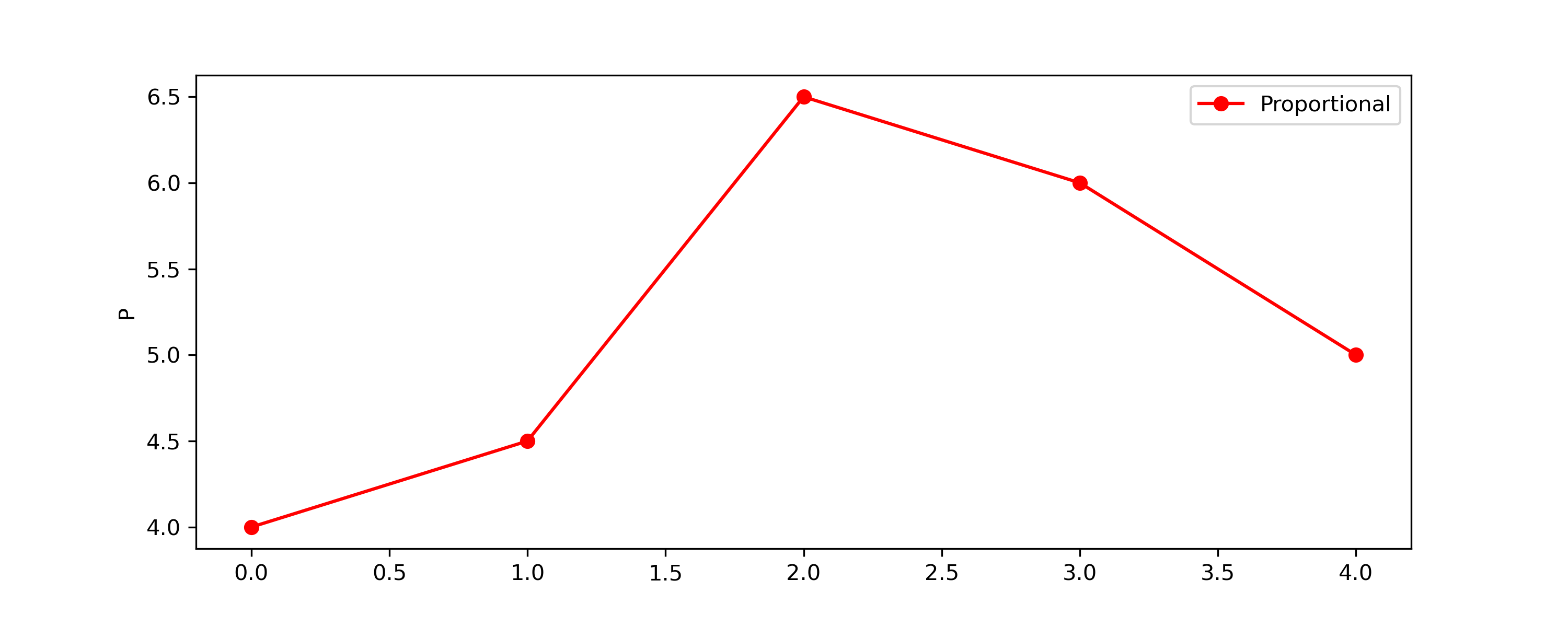
0	P	Proportional	4.0
1	P	Proportional	4.5
2	P	Proportional	6.5
3	P	Proportional	6.0
4	P	Proportional	5.0

Create a plot of the Proportional term P to show how it has changed.

plt.plot(t5['hist'],'r-o',label=t5['desc'].iloc[0])
plt.legend(); plt.ylabel(t5['tag'].iloc[0]); plt.show()

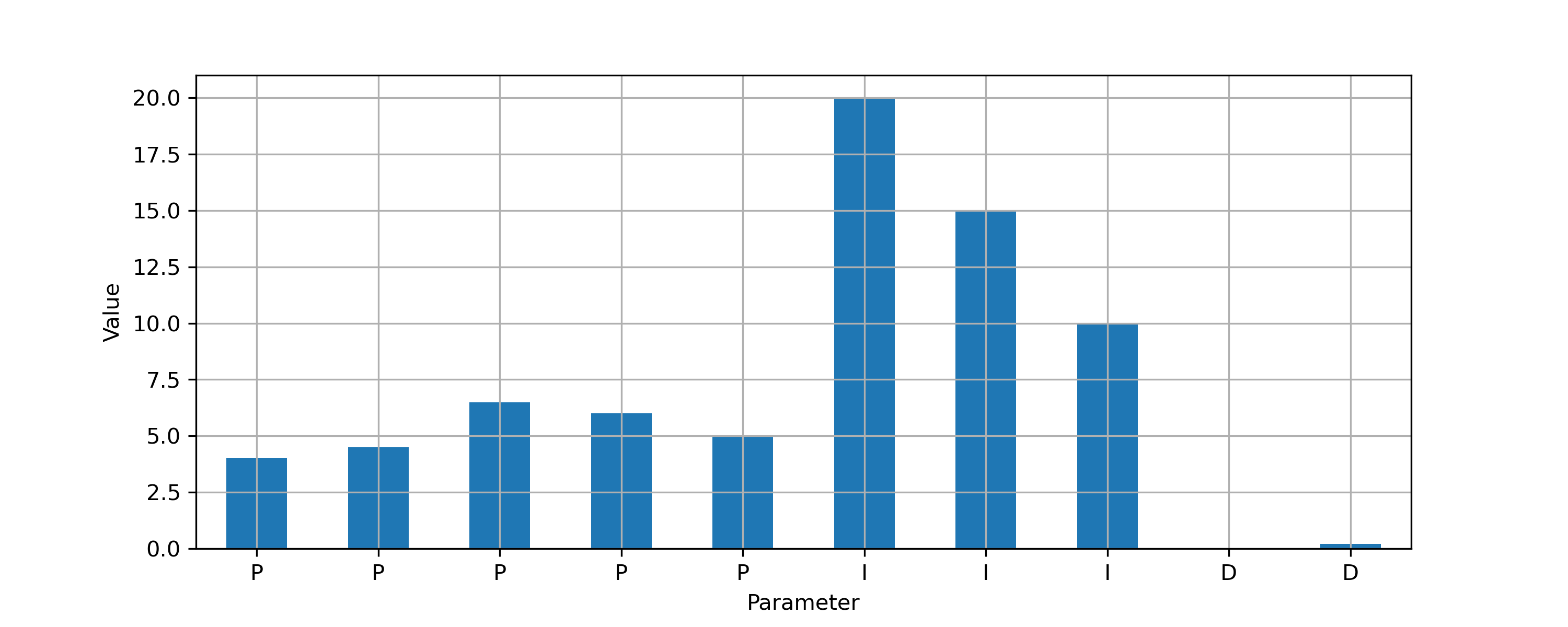
The table merge can also be completed with Pandas with the history of P, I and D shown on a single plot.

!join tables
t5 = t1.join(t2['desc'],on='id').join(t4['hist'],on='id')
!plot values
t5['hist'].plot(kind='bar')
plt.xticks(np.arange(0,len(t5)),t5['tag'],rotation='horizontal')
plt.ylabel('Value'); plt.xlabel('Parameter'); plt.grid()
!filter table to show only 'P' values
t5[t5['tag']=='P']

	tag	val	desc	hist
id
0	P	5.0	Proportional	4.0
0	P	5.0	Proportional	4.5
0	P	5.0	Proportional	6.5
0	P	5.0	Proportional	6.0
0	P	5.0	Proportional	5.0

✅ Activity

Create a new table t0 that contains 3 SQLite datatypes.

opID - Operator ID as integer (primary key)
name - Operator name as text (required)
photo - Operator profile photo as blob (optional)

New records (rows) will be added later. Use DROP TABLE IF EXISTS t0 to drop the table if it already exists.

cur.execute('DROP TABLE IF EXISTS t0')

Create the table t0 and insert records:

opID: 1 name: David Stevens
opID: 2 name: Rebecca Okume
opID: 3 name: Mike Fisher

Commit the changes once the records are added.

The new table t0 can now to be used to record details of who made the changes to the PID parameters by recording the opID in t4 when a new row is added to the history. It is not required to add a photo or augment t4 for this activity.

cur.execute('CREATE TABLE t0 (opID int PRIMARY KEY, \
name text NOT NULL)')
cmd = 'INSERT INTO t0 (opID, name) VALUES (?, ?)'
cur.execute(cmd, (1,'David Stevens'))
cur.execute(cmd, (2,'Rebecca Okume'))
cur.execute(cmd, (3,'Mike Fisher'))
cxn.commit()

Close Database Connection

Close the database connection with cxn.close(). This releases the database so that it prevents a connection after it is closed.

cxn.close()

✅ Knowledge Check

1. Which SQL statement is used to add rows to a table in a relational database?

A. DROP TABLE

Incorrect. DROP TABLE is used to delete a table from the database.

B. SELECT

Incorrect. SELECT is used to fetch rows from a table.

C. INSERT INTO

Correct. INSERT INTO is used to add rows to a table.

D. UPDATE

Incorrect. UPDATE is used to modify existing rows in a table.

2. What is the main difference between SQLite and other SQL databases?

A. SQLite does not use SQL

Incorrect. SQLite does use SQL. It is a minimal version of SQL.

B. SQLite can only store text data

Incorrect. SQLite supports various datatypes including int, real, text, and blob.

C. SQLite stores the entire database in one file or in memory

Correct. SQLite stores the entire database in a single file or in memory, making it suitable for small projects or on-device storage.

D. SQLite requires a server setup

Incorrect. SQLite doesn't require a server setup. It's serverless, zero-configuration, and self-contained.

Options:

fixed
fluid

orange
blue
green
pink
cyan
red
violet