State Space Model
State space models are a type of mathematical model that is used to describe the behavior of dynamic systems. These models are used in many fields, including engineering, economics, and physics. State space models are based on the concept of a state vector, which is a set of variables that represent the internal state of a system. In a state space model, the state vector is used to describe how the system evolves over time. This is done using a set of differential equations, known as the state equations, which describe how the state vector changes as a function of time.
In addition to the state equations, a state space model also includes an output equation, which describes how the state vector is related to the output of the system. This allows the model to be used to predict the output of the system for a given set of inputs. Overall, state space models are a useful tool for modeling and analyzing dynamic systems. They provide a compact and flexible way to describe the behavior of a system, and can be used to design control systems.
State space models can be in either discrete or continuous time. Putting a model into state space form is the basis for many methods in theory and application. Below is the continuous time form of a model in state space form.
$$\dot x = A x + B u$$
$$y = C x + D u$$
with states `x in \mathbb{R}^n` and state derivatives `\dot x = {dx}/{dt} in \mathbb{R}^n`. The notation `in \mathbb{R}^n` means that `x` and `\dot x` are in the set of real-numbered vectors of length `n`. The other elements are the outputs `y in \mathbb{R}^p`, the inputs `u in \mathbb{R}^m`, the state transition matrix `A`, the input matrix `B`, and the output matrix `C`. The remaining matrix `D` is typically zeros because the inputs do not typically affect the outputs directly. The dimensions of each matrix are shown below with `m` inputs, `n` states, and `p` outputs.
$$A \in \mathbb{R}^{n \, \mathrm{x} \, n}$$ $$B \in \mathbb{R}^{n \, \mathrm{x} \, m}$$ $$C \in \mathbb{R}^{p \, \mathrm{x} \, n}$$ $$D \in \mathbb{R}^{p \, \mathrm{x} \, m}$$
First Order System in State Space
The state space form can be difficult to grasp at first so consider an example to transform a first order linear system into state space form.
$$\frac{dy}{dt} = -y + 2 u$$
Add the output relationship `x = y` and `\dot x = \dot y` to give the following in state space form.
$$\dot x = [-1] x + [2] u$$
$$y = [1] x + [0] u$$
Second Order System in State Space
A second order linear system has `x in \mathbb{R}^2`, `y in \mathbb{R}^1`, `u in \mathbb{R}^1`, `A in \mathbb{R}^{2x2}`, `B in \mathbb{R}^{2x1}`, `C in \mathbb{R}^{1x2}` and `D in \mathbb{R}^{1x1}`. A second order overdamped system can be expressed as two first order linear systems in series.
$$\frac{dx_1}{dt} = -x_1 + 2 u$$
$$\frac{dx_2}{dt} = -x_2 + x_1$$
$$y = x_2$$
This gives the following in state space form.
$$\begin{bmatrix}\dot x_1\\\dot x_2\end{bmatrix} = \begin{bmatrix}-1&0\\1&-1\end{bmatrix} \begin{bmatrix}x_1\\x_2\end{bmatrix} + \begin{bmatrix}2\\0\end{bmatrix} u$$
$$y = \begin{bmatrix}0 & 1\end{bmatrix} \begin{bmatrix}x_1\\x_2\end{bmatrix} + \begin{bmatrix}0\end{bmatrix} u$$
Exercise
Put the following equations into state space form by determining matrices A, B, C, and D.
$$\dot x = A x + B u$$ $$y = C x + D u$$
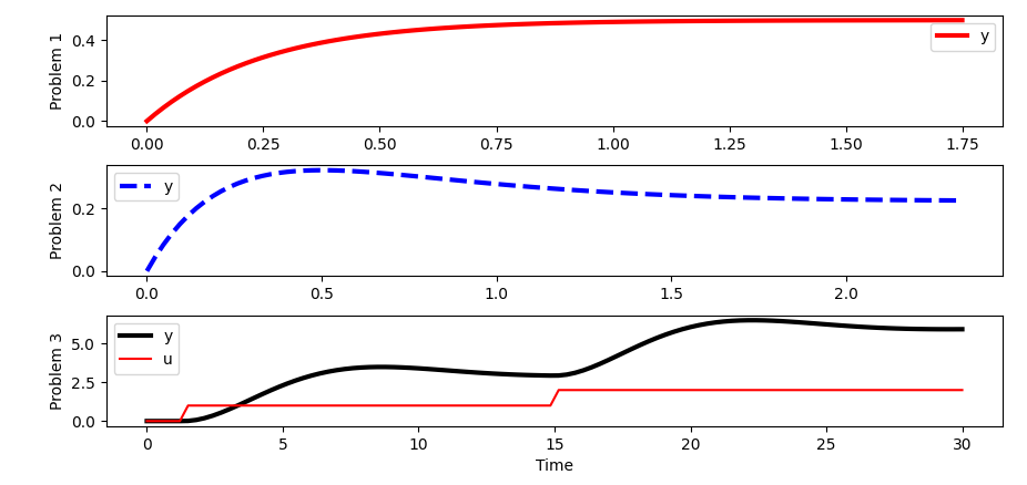
Simulate a step response for each model.
1. First order differential equation
$$3 \, \frac{dx}{dt} + 12 \, x = 6 \, u$$ $$y = x$$
2. Second order differential equations
$$2 \frac{dx_1}{dt} + 6 \, x_1 = 8 \, u$$ $$3 \frac{dx_2}{dt} + 6 \, x_1 + 9 \, x_2 = 0$$ $$y = \frac{x_1 + x_2}{2}$$
3. Second order differential equation
$$4 \frac{d^2y}{dt^2} + 2 \frac{dy}{dt} + y = 3 \, u$$
Solution
from scipy import signal
# problem 1
A = [-4.0]
B = [2.0]
C = [1.0]
D = [0.0]
sys1 = signal.StateSpace(A,B,C,D)
t1,y1 = signal.step(sys1)
# problem 2
A = [[-3.0,0.0],[-2.0,-3.0]]
print(np.linalg.eig(A)[0])
B = [[4.0],[0.0]]
C = [0.5,0.5]
D = [0.0]
sys2 = signal.StateSpace(A,B,C,D)
t2,y2 = signal.step(sys2)
# problem 3
A = [[0.0,1.0],[-0.25,-0.5]]
print(np.linalg.eig(A)[0])
B = [[0.0],[0.75]]
C = [1.0,0.0]
D = [0.0]
sys3 = signal.StateSpace(A,B,C,D)
t = np.linspace(0,30,100)
u = np.zeros(len(t))
u[5:50] = 1.0 # first step input
u[50:] = 2.0 # second step input
t3,y3,x3 = signal.lsim(sys3,u,t)
import matplotlib.pyplot as plt
plt.figure(1)
plt.subplot(3,1,1)
plt.plot(t1,y1,'r-',linewidth=3)
plt.ylabel('Problem 1')
plt.legend(['y'],loc='best')
plt.subplot(3,1,2)
plt.plot(t2,y2,'b--',linewidth=3)
plt.ylabel('Problem 2')
plt.legend(['y'],loc='best')
plt.subplot(3,1,3)
plt.plot(t3,y3,'k-',linewidth=3)
plt.plot(t,u,'r-')
plt.ylabel('Problem 3')
plt.legend(['y','u'],loc='best')
plt.xlabel('Time')
plt.show()
Sure, I'll start by posing two questions based on the content provided and will then shuffle the responses for correctness using the template.
✅ Knowledge Check
1. Which of the following statements about state space models is true?
- Incorrect. State space models are used to describe dynamic systems, not static ones.
- Correct. Indeed, the state vector describes the internal state of a system and how it changes over time.
- Incorrect. The output equation describes the relationship between the state vector and the system's output. It's the state equations that describe the change of the state vector over time.
- Incorrect. State space models are widely used in various fields, including engineering.
2. Consider the state space representation of the second order overdamped system. What can be said about the matrix D?
- Correct. Matrix D represents the direct effect of the inputs on the outputs. In the provided model, D is a zero matrix, meaning inputs don't directly affect outputs.
- Incorrect. Matrix D in the provided model is a 1x1 matrix with value zero.
- Incorrect. Matrix D is often zero, especially when inputs do not directly affect outputs.
- Incorrect. Matrix C is the output matrix. Matrix D represents the direct relationship between inputs and outputs.