Smartphone Sensors
Modern smartphones come equipped with a wide array of sensors that enhance the user experience and enable various functionalities. These sensors fall into several categories: motion, environmental, positional, biometric, and proximity sensors.
Motion Sensors
Motion sensors like accelerometers and gyroscopes enable dynamic functions. The accelerometer detects changes in motion and orientation across three axes, allowing automatic screen rotation and step counting. The gyroscope offers more precise motion detection, essential for gaming and augmented reality applications.
Environmental Sensors
Environmental sensors include barometers, thermometers, and ambient light sensors. The barometer measures atmospheric pressure, helping determine altitude and enhance GPS accuracy. Thermometers monitor device temperature to prevent overheating, while ambient light sensors adjust screen brightness based on ambient light, improving visibility and conserving battery life.
Positional Sensors
Positional sensors, such as magnetometers and GPS modules, provide orientation and precise location data. The magnetometer functions as a digital compass, while the GPS module communicates with satellites to provide location data, essential for navigation and location-based services.
Biometric Sensors
Biometric sensors, including fingerprint scanners and facial recognition systems, offer secure authentication. Fingerprint scanners use capacitive or ultrasonic technology for secure access, while facial recognition uses infrared sensors and cameras for hands-free unlocking.
Proximity Sensors
Proximity sensors detect nearby objects without physical contact, often used to turn off the display during phone calls when held near the ear, preventing accidental touches.
Applications of Smartphone Sensors
- Navigation and Mapping - GPS and magnetometers enable precise location tracking and navigation.
- Health and Fitness - Accelerometers and biometric sensors track physical activity and health metrics.
- Gaming and Augmented Reality - Gyroscopes and accelerometers enhance interactive gaming experiences.
- Photography - Ambient light sensors and motion data help adjust camera settings and stabilize images.
- Security - Biometric sensors provide secure authentication.
- Environmental Monitoring - Barometers and thermometers measure atmospheric pressure and temperature, useful for weather forecasting.
Smartphones, through these sensors, have transformed into versatile tools capable of performing many tasks beyond traditional communication.
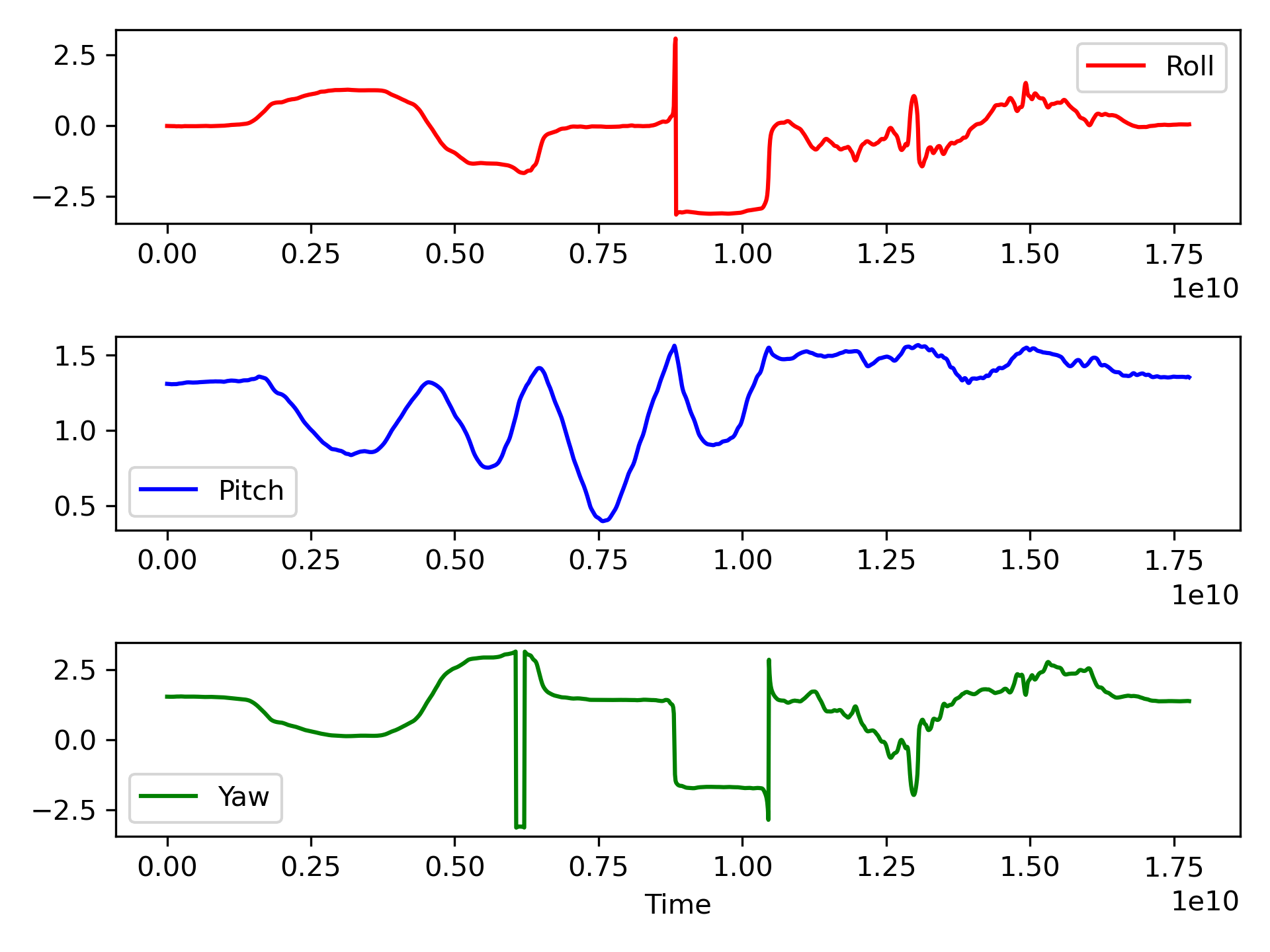
✅ Activity: Orientation
Objective: Use a smartphone to record orientation data (roll, pitch, and yaw) and then import and visualize this data in Python. Gain experience in data collection, CSV handling, and plotting in Python.
Install a Sensor Logger App
Data Collection
- Open the Sensor Logger app.
- Select the orientation sensor to log data for roll, pitch, and yaw.
- Start logging and carefully tilt the phone in various directions to capture orientation changes. Continue recording for about 1-2 minutes.
- Save the data and export it as a CSV file from the app.
- Transfer the CSV file from your phone to your computer.
- Open Python and load the data using pandas. Here is sample code to get started:
import matplotlib.pyplot as plt
# Load the CSV file
file = 'Orientation.csv'
try:
data = pd.read_csv(file)
except:
# data file not available, load online file
url = 'http://apmonitor.com/dde/uploads/Main/'
data = pd.read_csv(url+file)
# Cleanse data
data['time'] = (data['time'] - data['time'].iloc[0])/1e9
# Plot roll, pitch, and yaw
plt.figure(figsize=(6,4))
plt.subplot(3,1,1)
plt.plot(data['time'], data['roll'], color='red', label='Roll')
plt.legend()
plt.subplot(3,1,2)
plt.plot(data['time'], data['pitch'], color='blue', label='Pitch')
plt.legend()
plt.subplot(3,1,3)
plt.plot(data['time'], data['yaw'], color='green', label='Yaw')
plt.legend()
plt.xlabel('Time (sec)')
plt.tight_layout()
plt.show()
Analysis
Display roll, pitch, and yaw data over time, visualizing the smartphone orientation. Observe any patterns observed in the data. For instance, identify how roll, pitch, and yaw change as the phone orientation varies. This activity teaches data handling and plotting in Python and provides insight into sensor data collection.
✅ Activity: Vibration
Consider how vibration data (acceleration) may be applied in applications like rotating equipment monitoring. Place the phone on a flat surface and start recording. Alternate 5 second periods of tapping the table to induce vibration over about 20 seconds. Plot and analyze the data to show how an accelerometer could be applied to detect excessive vibration from rotating equipment such as a motor or pump.
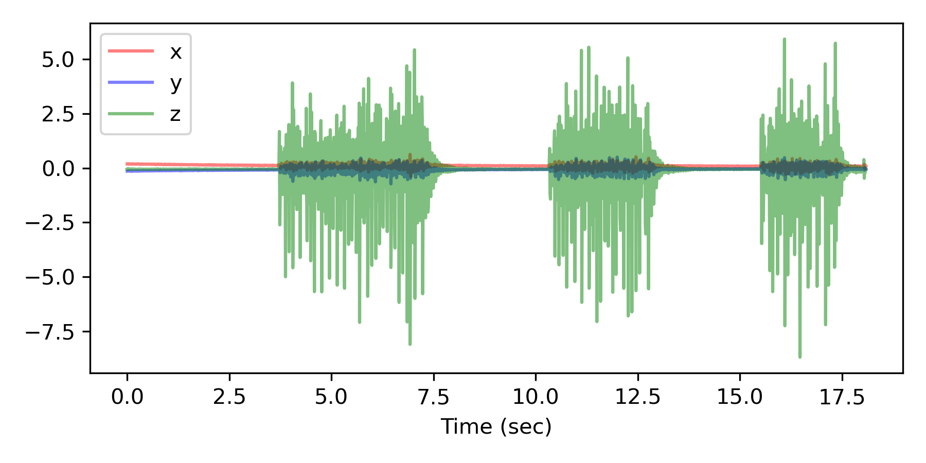
import matplotlib.pyplot as plt
# Load the CSV file
file = 'Accelerometer.csv'
try:
data = pd.read_csv(file)
except:
# data file not available, load online file
url = 'http://apmonitor.com/dde/uploads/Main/'
data = pd.read_csv(url+file)
# Cleanse data
data['time'] = (data['time'] - data['time'].iloc[0])/1e9
# Plot x,y,z acceleration
plt.figure(figsize=(6,3))
plt.plot(data['time'], data['x'], color='red', label='x', alpha=0.5)
plt.plot(data['time'], data['y'], color='blue', label='y', alpha=0.5)
plt.plot(data['time'], data['z'], color='green', label='z', alpha=0.5)
plt.legend()
plt.xlabel('Time (sec)')
plt.tight_layout()
plt.show()
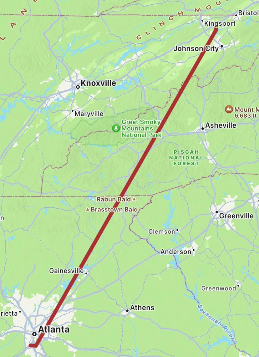
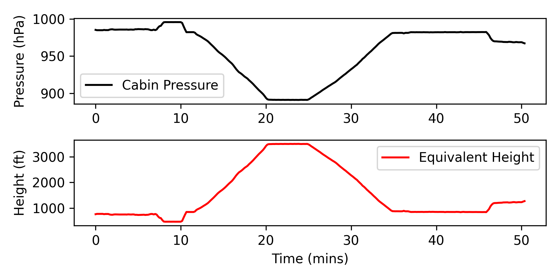
✅ Activity: Cabin Pressure During Flight
Objective: Record and analyze the pressure inside an airplane cabin from takeoff to landing. This activity uses the smartphone barometer sensor to monitor pressure changes during the ascent, cruise, and descent of a flight. The sample demonstration data is for a commercial flight between Atlanta, GA and Tri-Cities, TN.
The difference in elevation is observable as a change in pressure between the two airports and can be used to check the beginning and ending pressures. Atmospheric conditions cause natural variation in the pressure at the same altitude. See the relationships between air pressure and elevation with the BMP280 sensor material.
Data Collection
- Select the barometer in the Sensor Logger app to measure pressure.
- Begin logging data at 10 sec intervals before the aircraft door is closed and continue during the flight. Stop after landing and the aircraft door is opened.
- Save the data as a CSV file and transfer it from the smartphone to a computer.
Additional Information on Elevation
- Hartsfield-Jackson Atlanta International Airport is at an elevation of 1,026 feet above sea level.
- Tri-Cities, TN Airport is located at an elevation of 1,519 feet above sea level.
import matplotlib.pyplot as plt
# Load the CSV file
file = 'Barometer.csv'
try:
data = pd.read_csv(file)
except:
# data file not available, load online file
url = 'http://apmonitor.com/dde/uploads/Main/'
data = pd.read_csv(url+file)
# Cleanse data
data['time'] = (data['time'] - data['time'].iloc[0])/60e9
# Equivalent height
T0 = 288.16; L=0.00976; P0=1013.25; Rg=8.31446
g = 9.80665; M=0.02896968
data['h'] = (T0/L)*(1-(data['pressure']/P0)**(Rg*L/(g*M))) * 3.28084
# Plot cabin pressure and equivalent height over time
plt.figure(figsize=(6,3))
plt.subplot(2,1,1)
plt.plot(data['time'], data['pressure'], 'k-', label='Cabin Pressure')
plt.ylabel('Pressure (hPa)'); plt.legend()
plt.subplot(2,1,2)
plt.plot(data['time'], data['h'], 'r-', label='Equivalent Height')
plt.ylabel('Height (ft)'); plt.legend()
plt.xlabel('Time (mins)')
plt.tight_layout()
plt.show()
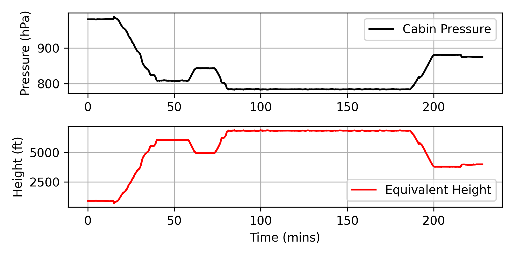
Additional Information on Elevation
- Hartsfield-Jackson Atlanta International Airport is at an elevation of 1,026 feet above sea level.
- Salt Lake City International Airport is located at an elevation of 4,226 feet above sea level.
import matplotlib.pyplot as plt
# Load the CSV file
file = 'Barometer2.csv'
url = 'http://apmonitor.com/dde/uploads/Main/'
data = pd.read_csv(url+file)
# Cleanse data
data['time'] = (data['time'] - data['time'].iloc[0])/60e9
# Equivalent height
T0 = 288.16; L=0.00976; P0=1013.25; Rg=8.31446
g = 9.80665; M=0.02896968
data['h'] = (T0/L)*(1-(data['pressure']/P0)**(Rg*L/(g*M))) * 3.28084
# Plot cabin pressure and equivalent height over time
plt.figure(figsize=(6,3))
plt.subplot(2,1,1)
plt.plot(data['time'], data['pressure'], 'k-', label='Cabin Pressure')
plt.ylabel('Pressure (hPa)'); plt.grid(); plt.legend()
plt.subplot(2,1,2)
plt.plot(data['time'], data['h'], 'r-', label='Equivalent Height')
plt.ylabel('Height (ft)'); plt.legend()
plt.xlabel('Time (mins)'); plt.grid()
plt.tight_layout()
plt.show()
✅ Exercise: Floor Detection
Modern smartphones are equipped with multiple sensors that can collect physical and environmental data. This assignment provides hands-on experience in identifying, recording, and analyzing data from these sensors using your smartphone and Python.
Part 1: Sensor Inventory
Objective: Identify and document the sensors available on your smartphone.
Instructions:
- Open the Sensor Logger app on your smartphone.
- Explore the list of available sensors.
- Create a table summarizing your phone’s sensors. For each sensor, include:
- Sensor Type (e.g., Accelerometer, Gyroscope, Barometer)
- Quantity Recorded (e.g., 3-axis acceleration)
- Units (e.g., m/s², °C, hPa)
- Typical Range of Values (observed from exported CSV data)
- Save your table as part of your report.
Example Table (HTML):
| Sensor Type | Quantity Recorded | Units | Range (Example) |
|---|---|---|---|
| Accelerometer | x, y, z | m/s² | -9.8 to +9.8 |
| Gyroscope | x, y, z | deg/s | -180 to +180 |
| Barometer | pressure | hPa | 960–1020 |
| Ambient Light | intensity | lx | 0–50,000 |
| Magnetometer | x, y, z | µT | -60 to +60 |
| Thermometer (device) | temperature | °C | 20–60 (device-dependent) |
Part 2: Barometer Experiment – Detecting Floors
Objective: Use the barometer sensor to detect altitude changes while walking up or down multiple floors.
Instructions:
- In the Sensor Logger app, select the Barometer sensor.
- Start logging while standing on the ground floor of a multi-story building.
- Walk up and down several floors (or take the elevator). Important Safety Information: Use handrails, focus on walking (don't look at phone while moving).
- Stop recording after returning to your starting point.
- Export the logged data as a CSV file and transfer it to your computer as barometer.csv.
import matplotlib.pyplot as plt
# Load the CSV file
file = 'Barometer.csv'
data = pd.read_csv(file)
# Cleanse data
data['time'] = (data['time'] - data['time'].iloc[0]) / 1e9
# Convert pressure (kPa) to equivalent height (m)
T0 = 288.16; L = 0.00976; P0 = 1013.25; Rg = 8.31446
g = 9.80665; M = 0.02896968
data['height'] = (T0 / L) * (1 - (data['pressure'] / P0)**(Rg * L / (g * M)))
# Plot pressure and equivalent height
plt.figure(figsize=(6,3))
plt.subplot(2,1,1)
plt.plot(data['time'], data['pressure'], 'k-', label='Pressure')
plt.ylabel('Press (hPa)')
plt.legend(); plt.grid()
plt.subplot(2,1,2)
plt.plot(data['time'], data['height'], 'r-', label='Height (m)')
plt.legend(); plt.grid()
plt.ylabel('Height (m)')
plt.xlabel('Time (s)')
plt.tight_layout()
plt.show()
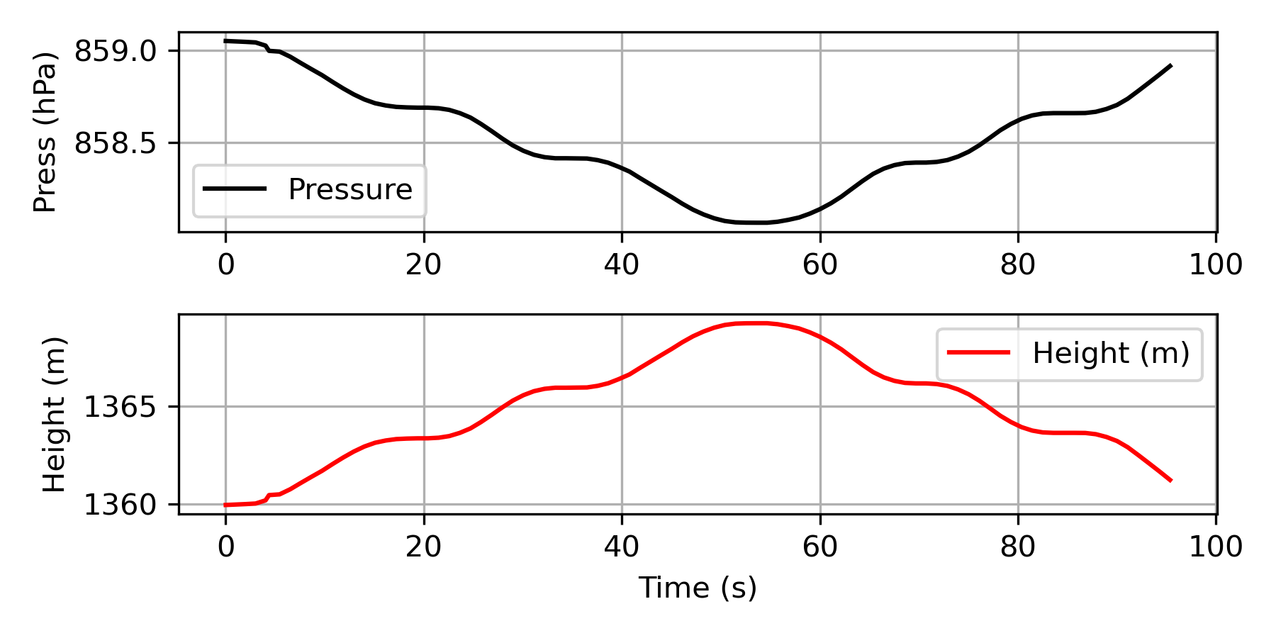
Analysis Questions:
- How much did the pressure change per floor?
- Estimate the altitude difference between two floors.
- Can you detect how many floors you climbed or descended?
- Compare your pressure-based height change with the known floor spacing.
Discussion
Reflect on your findings:
- How accurate are smartphone sensors for detecting altitude?
- What are potential real-world uses for this type of data (e.g., fitness tracking, building monitoring, emergency response)?
- Discuss any sources of error or limitations in the data.
What to Turn In
- A brief introduction (2–3 sentences) on smartphone sensors.
- Sensor Inventory Table from Part 1.
- A plot of pressure and equivalent height vs. time from Part 2.
- Answers to the analysis and discussion questions.
- The CSV data files from your smartphone (orientation and barometer experiments).
- Python script or Jupyter Notebook used to generate the plots.
✅ Exercise: Multiple Smartphone Sensors
Modern smartphones can record data from many sensors simultaneously, but each sensor is often saved to a separate CSV file with different sampling rates and missing values. In this exercise, you will combine multiple sensor CSV files into a single dataset and visualize selected sensors over time.
Objective
- Combine multiple sensor CSV files into a single pandas DataFrame
- Align sensor data using time as a common index
- Forward-fill missing values caused by different sensor sampling rates
- Select sensors of interest and visualize their data
- Identify and remove rows with bad or incomplete data (student task)
- Create time-series plots of the cleaned data (student task)
Data Collection
- Use the Sensor Logger app to record data from multiple sensors at the same time (e.g., Accelerometer, Gyroscope, Orientation, Barometer).
- Start all selected sensors simultaneously.
- Record data for ~1 minute while moving the phone (walking, rotating, or placing it on a surface).
- Stop logging and export all sensor data as CSV files.
- Transfer all CSV files into the same folder on your computer.
Part 1: Combine Sensor CSV Files
Use the provided Python script to:
- Load all sensor CSV files in a folder
- Align them by time
- Forward-fill missing values
- Create a single combined DataFrame and CSV
from pathlib import Path
# Folder containing sensor CSV files
folder = Path('./data') # change if needed
dfs = []
loaded = []
for file in sorted(folder.glob('*.csv')):
# 1) Skip empty files (prevents EmptyDataError)
if file.stat().st_size == 0:
print(f"Skipping empty file: {file.name}")
continue
# 2) Try reading; skip files that still have no parsable columns
try:
data = pd.read_csv(file)
except pd.errors.EmptyDataError:
print(f"Skipping unreadable/empty CSV: {file.name}")
continue
except Exception as e:
print(f"Skipping {file.name} (read error: {e})")
continue
# 3) Must contain a 'time' column to be a sensor file
if 'time' not in data.columns:
print(f"Skipping {file.name} (no 'time' column)")
continue
# 4) Ensure time is numeric and drop bad time rows
data['time'] = pd.to_numeric(data['time'], errors='coerce')
data = data.dropna(subset=['time']).copy()
if len(data) == 0:
print(f"Skipping {file.name} (no valid time rows)")
continue
# 5) Drop seconds_elapsed if present (optional)
if 'seconds_elapsed' in data.columns:
data = data.drop(columns=['seconds_elapsed'])
# 6) Use time as index and sort
data = data.set_index('time').sort_index()
# 7) If duplicate timestamps, keep last
data = data[~data.index.duplicated(keep='last')]
dfs.append(data)
loaded.append(file.name)
if not dfs:
raise RuntimeError("No sensor CSV files found.")
# Combine all sensors and forward-fill missing values
combined = pd.concat(dfs, axis=1).sort_index().ffill()
print("\nLoaded sensor files:")
for f in loaded:
print(" -", f)
print("\nCombined shape:", combined.shape)
print(combined.head())
# Optional: save it
combined.to_csv("combined.csv")
print("\nWrote combined.csv")
Part 2: Sensor Selection and Visualization
- Choose at least two different sensors (e.g., accelerometer and gyroscope).
- Identify which columns correspond to your selected sensors.
- Create plots of the selected sensor variables versus time.
Part 3: Data Cleaning (Student Task)
Many rows in the combined dataset may contain missing or unreliable data due to:
- Different sensor sampling rates
- Sensor dropouts
- Initialization delays
Your task:
- Identify rows with missing data
- Remove or filter these rows
Part 4: Time-Series Plotting (Student Task)
After cleaning the data:
- Create time-series plots of the selected sensors
- Use consistent time axes
- Label plots (units, sensor names, legends)
Analysis Questions
- Why do different sensors produce missing data when logged simultaneously?
- How does forward-filling affect the interpretation of sensor signals?
- What are the risks of removing too much data during cleaning?
- Which sensors would be useful to detect a automobile crash?
What to Turn In
- A brief description of the sensors you selected
- The combined CSV file
- Your cleaned DataFrame
- Time-series plots of the selected sensors
- A short explanation of how you handled missing or bad data
- The Python script or Jupyter Notebook used in your analysis