Time-Series to Image


Converting time-series data into images caters both to human intuition and advanced machine learning techniques. For humans, visual representations distill complex data patterns into easily interpretable forms, enabling quicker insights and more intuitive understanding of underlying trends and anomalies. On the machine learning front, this transformation unlocks the potential of powerful image-based classifiers, especially Convolutional Neural Networks (CNNs) to extract hierarchical features from images for classification. This conversion of time-series data to an image aids in direct visual analysis and facilitates sophisticated, image-driven machine learning applications, using the strengths of human cognition and computational power.
Spectrogram from Audio Data
Audio data is a time-series of frequency information that is recorded from a sound signal. A spectrogram is a visual representation of the spectrum of frequencies in a sound or other signal as they vary with time. The matplotlib and scipy libraries in Python provide tools to generate a spectrogram. See Audio Analysis for an application of detecting a nearby drone from a spectrogram of audio data.
import matplotlib.pyplot as plt
from scipy.signal import spectrogram
# Sample data: Generate a signal
fs = 10e3
t = np.arange(0, 1.0, 1.0/fs)
x = np.sin(2*np.pi*3e3*t) + 0.5*np.sin(2*np.pi*1e3*t)
frequencies, times, Sxx = spectrogram(x, fs)
plt.pcolormesh(times, frequencies, 10 * np.log10(Sxx), shading='gouraud')
plt.colorbar(label='Intensity [dB]')
plt.ylabel('Frequency [Hz]')
plt.xlabel('Time [sec]')
plt.show()
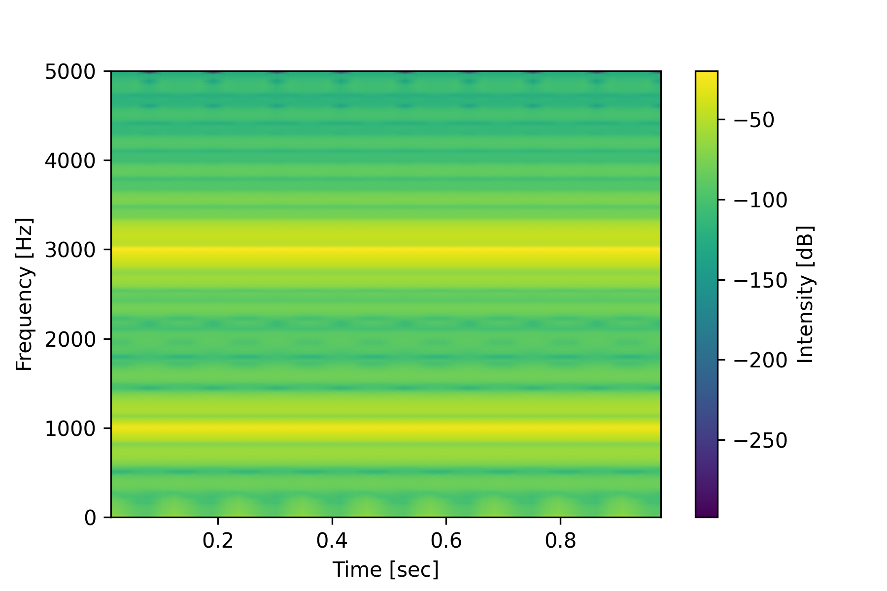
Image from ECG Data
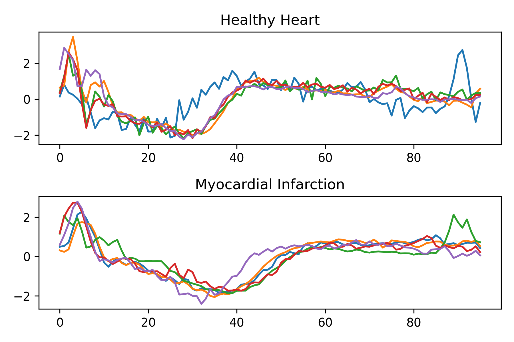
Electrocardiogram (ECG) data represents the electrical activity of the heart over time. Visualizing the heat beat cycle can discern patterns that indicate heart health. The Aeon library has sample time-series data available for easy retrieval. The code imports necessary functions from the aeon.datasets module. It then retrieves the ECG200 dataset as a collection of ECG heart readings. This dataset is from the thesis:
Each series traces the electrical activity recorded during one heartbeat. The two classes are a normal heartbeat and a myocardial infarction (heart attack). The dataset is loaded into three variables: X (ECG readings), y (heart health), and meta_data that describes the dataset.
from aeon.datasets import load_classification
X, y, meta_data = load_classification("ECG200")
print(" Shape of X = ", X.shape)
print(" Meta data = ", meta_data)
#visualize data
for i in range(10):
if int(y[i])>0:
plt.subplot(2,1,1)
plt.plot(X[i,0,:])
else:
plt.subplot(2,1,2)
plt.plot(X[i,0,:])
plt.subplot(2,1,1)
plt.title('Healthy Heart')
plt.subplot(2,1,2)
plt.title('Myocardial Infarction')
plt.tight_layout()
plt.savefig('heart_health.png',dpi=300)
Preprocessing Functions
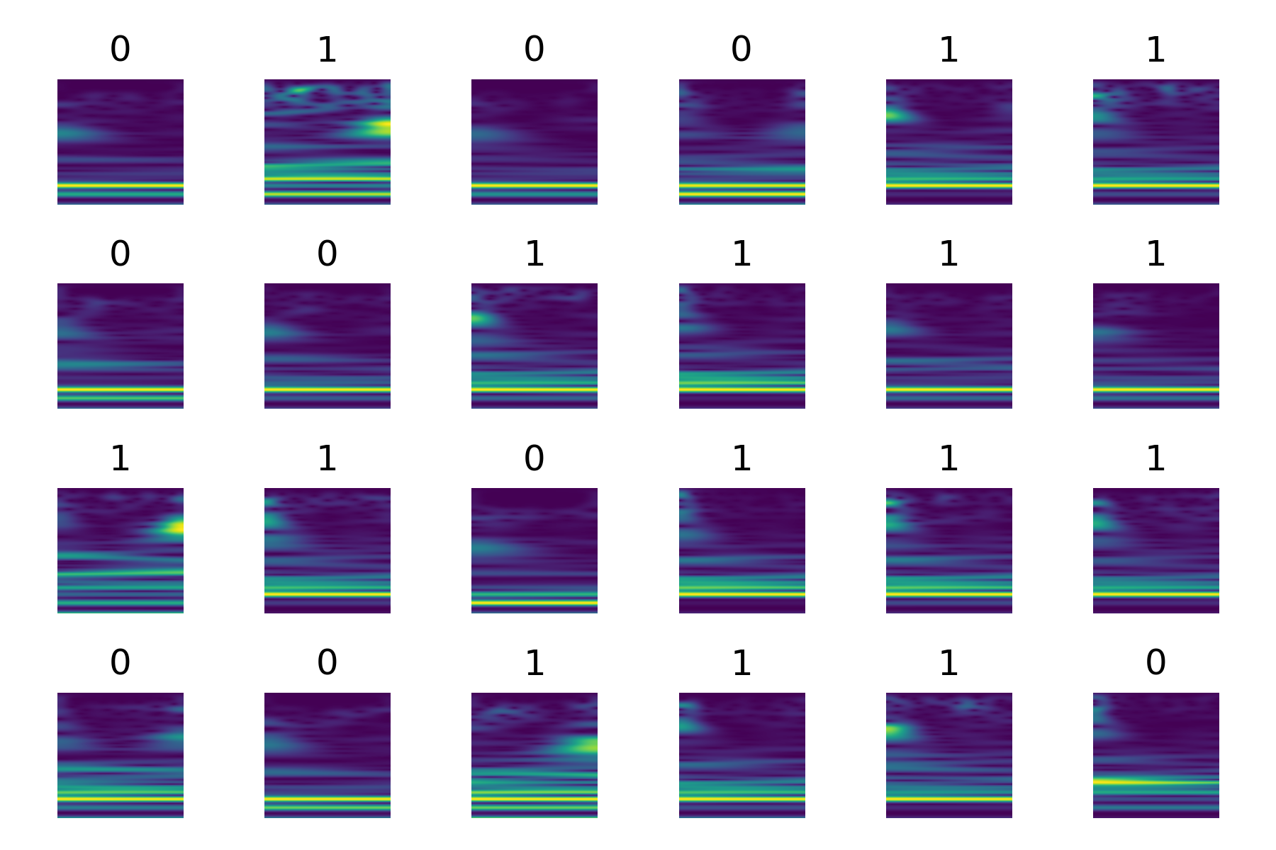
The following code provides a framework for preprocessing and organizing time-series data for use with a PyTorch deep learning model. Initially, the code imports necessary libraries from PyTorch, ssqueezepy for Continuous Wavelet Transforms (CWT), and sklearn for data preprocessing. The function CWT applies the continuous wavelet transform using the Generalized Morse wavelets, specifically the Morlet wavelet, to the provided signal and subsequently normalizes the result. The CustomDataset class structures the data such that it can be ingested by PyTorch's DataLoader. It inherits from PyTorch's Dataset class and implements methods to transform the data, retrieve individual data items, determine the dataset's length, and visualize the transformed time-series data as an image. This organized structure streamlines feeding the processed data into neural network models for training or inference.
from torch.utils.data import Dataset, DataLoader
from torchvision import transforms
from torch import nn
from torch import optim
from ssqueezepy import cwt
from sklearn import preprocessing
# CWT with Generalzied morse wavelets
def CWT(signal):
Wx,scales = cwt(signal,wavelet='morlet') #lots of options here
Wx = np.abs(Wx)
for i in range(Wx.shape[0]):
Wx[i,:,:] = (Wx[i,:,:] - Wx[i,:,:].min()) / (Wx[i,:,:].max() - Wx[i,:,:].min())
return Wx
# Organize Pytorch dataset into a structure that can be loaded into dataloaders
class CustomDataset(Dataset):
def __init__(self,X,y):
#transform
self.preprocess = transforms.Compose([
transforms.Resize((224,224),antialias=None)
])
self.X = X; self.y = y
def __getitem__(self,index):
Xi = self.X[index]; yi = self.y[index]
return self.preprocess(torch.tensor(CWT(Xi))),\
torch.tensor(yi).type(torch.LongTensor)
def __len__(self):
return len(self.X)
def show(self,index):
Xi,yi = self[index]
nXi = Xi.numpy()
plt.imshow(nXi[0])
Generate Image of ECG Data
The next step is to preprocess the set of labels (y) and visualize a subset of the dataset. The label array y contains values of either -1 or 1 and it transforms the labels to a more conventional range of 0 and 1. The LabelEncoder from sklearn.preprocessing performs this transformation to yt. The transformed data (X and yt) is used to visualize the first 24 entries of the train dataset. For each entry, a subplot is created in a grid layout of 4 rows by 6 columns.
le = preprocessing.LabelEncoder()
le.fit(y)
yt = le.transform(y)
train = CustomDataset(X, yt)
for i in range(24):
plt.subplot(4,6,i+1)
train.show(i)
plt.axis('off')
xi,yi = train[i]
plt.title(yi.numpy())
plt.tight_layout()
plt.savefig('heart_health2.png')
plt.show()
Activity

Stiction ("static" and "friction") of control valves is the resistance to start movement when a valve has been stationary for a period. The stiction can cause the valve to stick in the current position, requiring a sufficient signal change to start moving. Once the valve begins moving, it may move too much because of the excessive command given to overcome the stiction. This results in oscillations in the controlled process variable that aren't the result of normal loop oscillations. Such oscillations can look distinctive (saw-tooth) and can degrade process performance.
PID with Heater Stiction (10%)
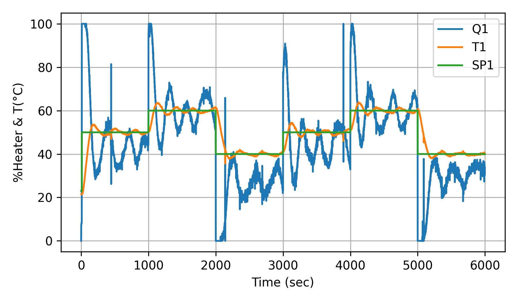
Well-tuned PID controller with heater stiction.
The objective of the Temperature Control Lab (TCLab) activity is to create images from the process data with and without simulated heater stiction similar to the example above for ECG data. Use a physical or simulated TCLab with PID control to regulate the temperature. Start with a constant setpoint and let the system achieve a steady state. The example images show set point changes. Introduce heater stiction by creating a simple programmatic minimum move in the heater response to the control signal. For instance, only change the heater power if the control signal changes by more than 10%.
if abs(Q1[i]-op_last)>stiction:
op_last = Q1[i]
Observe the temperature response and compare this with a response where the heater responds normally to the control signal. Collect time-series data for both scenarios with and without heater stiction.
PID Oscillating without Heater Stiction
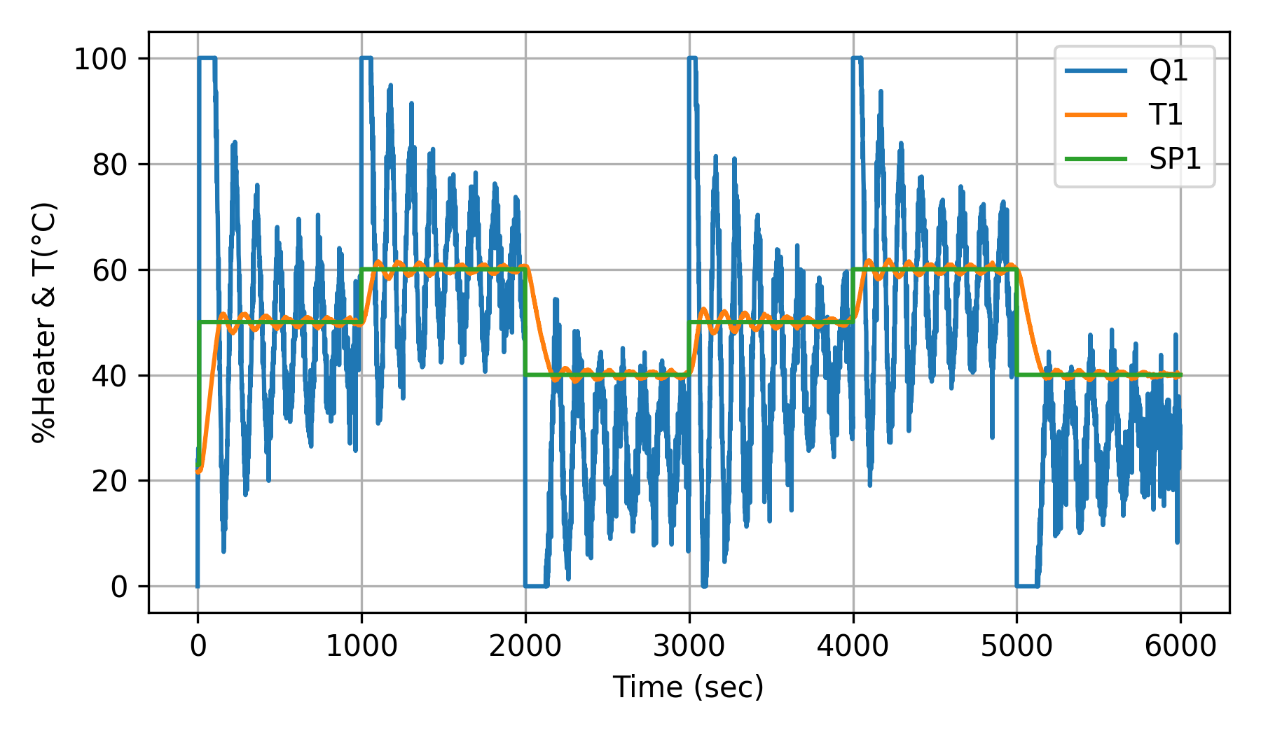
Poorly tuned PID controller response is similar to heater stiction.
Just as ECG data has distinctive patterns that correspond to healthy or unhealthy heart rhythms, the time-series data from the control lab shows distinctive cycles due to simulated heater stiction. Convert the time-series data (each cycle or a window of data) to images and observe the differences in images.
import numpy as np
import time
import matplotlib.pyplot as plt
from scipy.integrate import odeint
import pandas as pd
stiction = 10.0 # {0.0, 10.0}
tuning = 'moderate' # {'aggressive','moderate'}
######################################################
# PID Controller #
######################################################
# inputs -----------------------------------
# sp = setpoint
# pv = current temperature
# pv_last = prior temperature
# ierr = integral error
# dt = time increment between measurements
# outputs ----------------------------------
# op = output of the PID controller
# P = proportional contribution
# I = integral contribution
# D = derivative contribution
def pid(sp,pv,pv_last,ierr,dt):
if tuning=='aggressive':
# Aggressive Ocillating PID: Kc=15, tauI=30, tauD=1
# Moderate Ocillating PID: Kc=5, tauI=40, tauD=1
Kc = 15.0 # K/%Heater
tauI = 30.0 # sec
tauD = 1.0 # sec
else:
# Tuned PID: Kc=5, tauI=50, tauD=1
Kc = 5.0 # K/%Heater
tauI = 50.0 # sec
tauD = 1.0 # sec
# Parameters in terms of PID coefficients
KP = Kc
KI = Kc/tauI
KD = Kc*tauD
# ubias for controller (initial heater)
op0 = 0
# upper and lower bounds on heater level
ophi = 100
oplo = 0
# calculate the error
error = sp-pv
# calculate the integral error
ierr = ierr + KI * error * dt
# calculate the measurement derivative
dpv = (pv - pv_last) / dt
# calculate the PID output
P = KP * error
I = ierr
D = -KD * dpv
op = op0 + P + I + D
# implement anti-reset windup
if op < oplo or op > ophi:
I = I - KI * error * dt
# clip output
op = max(oplo,min(ophi,op))
# return the controller output and PID terms
return [op,P,I,D]
# save txt file with data and set point
# t = time
# u1,u2 = heaters
# y1,y2 = tempeatures
# sp1,sp2 = setpoints
def save_txt(t, u1, u2, y1, y2, sp1, sp2):
data = np.vstack((t, u1, u2, y1, y2, sp1, sp2)) # vertical stack
data = data.T # transpose data
top = ('Time,Q1,Q2,T1,T2,SP1,SP2')
np.savetxt('data.csv', data, fmt='%.3f', \
delimiter=',', header=top, comments='')
# Connect to Arduino
a = tclab.TCLab()
# Turn LED on
print('LED On')
a.LED(100)
# Run time in minutes
run_time = 100.0
# Number of cycles
loops = int(60.0*run_time)
tm = np.zeros(loops)
# Temperature
# set point (degC)
Tsp1 = np.ones(loops) * 23.0
Tsp1[10:] = 50.0
# Change to True to change setpoints
if False:
Tsp1[1000:] = 60.0
Tsp1[2000:] = 40.0
Tsp1[3000:] = 50.0
Tsp1[4000:] = 60.0
Tsp1[5000:] = 40.0
T1 = np.ones(loops) * a.T1 # measured T (degC)
Tsp2 = np.ones(loops) * 23.0 # set point (degC)
T2 = np.ones(loops) * a.T2 # measured T (degC)
# Heater (0 - 100%)
Q1 = np.ones(loops) * 0.0
Q2 = np.ones(loops) * 0.0
print('Running Main Loop. Ctrl-C to end.')
print(' Time SP PV Q1')
print(('{:6.1f} {:6.2f} {:6.2f} {:6.2f}').format( \
tm[0],Tsp1[0],T1[0],Q1[0]))
# Create plot
#plt.figure() #figsize=(10,7)
#plt.ion()
#plt.show()
# Main Loop
start_time = time.time()
prev_time = start_time
dt_error = 0.0
op_last = 0.0
# Integral error
ierr = 0.0
try:
for i in range(1,loops):
# Sleep time
sleep_max = 1.0
sleep = sleep_max - (time.time() - prev_time) - dt_error
if sleep>=1e-4:
time.sleep(sleep)
else:
print('exceeded max cycle time by ' + str(abs(sleep)) + ' sec')
time.sleep(1e-4)
# Record time and change in time
t = time.time()
dt = t - prev_time
if (sleep>=1e-4):
dt_error = dt-1.0+0.009
else:
dt_error = 0.0
prev_time = t
tm[i] = t - start_time
# Read temperatures in Kelvin
T1[i] = a.T1
T2[i] = a.T2
# Calculate PID output
[Q1[i],P,ierr,D] = pid(Tsp1[i],T1[i],T1[i-1],ierr,dt)
# simulate heater "stiction"
if abs(Q1[i]-op_last)>stiction:
op_last = Q1[i]
# Write output (0-100)
a.Q1(op_last)
a.Q2(0.0)
# Print line of data
print(('{:6.1f} {:6.2f} {:6.2f} {:6.2f}').format( \
tm[i],Tsp1[i],T1[i],Q1[i]))
if False:
# Plot
plt.clf()
ax=plt.subplot(2,1,1)
ax.grid()
plt.plot(tm[0:i],T1[0:i],'r.',label=r'$T_1$ measured')
plt.plot(tm[0:i],Tsp1[0:i],'k--',label=r'$T_1$ set point')
plt.ylabel('Temperature (degC)')
plt.legend(loc=2)
ax=plt.subplot(2,1,2)
ax.grid()
plt.plot(tm[0:i],Q1[0:i],'b-',label=r'$Q_1$')
plt.ylabel('Heater')
plt.legend(loc='best')
plt.xlabel('Time (sec)')
plt.draw()
plt.pause(0.05)
# Turn off heaters
a.Q1(0); a.Q2(0)
# Save text file
save_txt(tm[0:i],Q1[0:i],Q2[0:i],\
T1[0:i],T2[0:i],Tsp1[0:i],Tsp2[0:i])
# Save figure
data = pd.read_csv('data.csv')
data.set_index('Time',drop=True)
data[['Q1','T1','SP1']].plot(figsize=(6,3.5))
plt.xlabel('Time (sec)'); plt.ylabel('%Heater & T(°C)')
plt.tight_layout(); plt.grid()
plt.savefig('data.png',dpi=300)
plt.show()
# Allow user to end loop with Ctrl-C
except KeyboardInterrupt:
# Disconnect from Arduino
a.Q1(0)
a.Q2(0)
print('Shutting down')
a.close()
save_txt(tm[0:i],Q1[0:i],Q2[0:i],T1[0:i],T2[0:i],Tsp1[0:i],Tsp2[0:i])
#plt.savefig('test_PID.png',dpi=300)
# Make sure serial connection still closes when there's an error
except:
# Disconnect from Arduino
a.Q1(0)
a.Q2(0)
print('Error: Shutting down')
a.close()
save_txt(tm[0:i],Q1[0:i],Q2[0:i],T1[0:i],T2[0:i],Tsp1[0:i],Tsp2[0:i])
#plt.savefig('test_PID.png',dpi=300)
raise
Thanks to LaGrande Gunnell for the initial ECG example. Additional information on this method is available from: